1. Basic steps for pytorch to realize linear regression

1. Construct data set
2. Define Model function module
3. Construct the forward() function in the function module (that is, calculate y_pred)
4. Calculate loss value
5. Select optimization method
6. Training cycle iteration

2. Several optimization methods of pytorch

• Adagrad
• Adam
• Adamax
• ASGD
• LBFGS
• RMSprop
• Rprop
• SGD (random gradient descent)

3. Implementation of simple linear regression

Here we still y = 2 x y = 2x y=2x is realized as an example. The final iteration goal is w =2 and b =0. The selection learning rate is 0.01 and the initialization W is 1

The dataset is shown below

x_data = [1.0, 2.0, 3.0]
y_data = [2.0, 4.0, 6.0]

3.1 source code implementation

# -*- coding:utf-8 -8-
"""
Author: FeverTwice
Date: 2021--08--03
"""
import torch
import numpy as np
import matplotlib.pyplot as plt

x_data = torch.tensor([[1.0], [2.0], [3.0]])  # This must be a two-dimensional matrix
y_data = torch.tensor([[2.0], [4.0], [6.0]])


# Define function module
class LinearModel(torch.nn.Module):
    def __init__(self):
        super(LinearModel, self).__init__()  # Call the constructor of the parent class
        self.linear = torch.nn.Linear(1, 1)  # The two parameters passed in are w and b, which are automatically constructed

    def forward(self, x):
        y_pred = self.linear(x)
        return y_pred


model = LinearModel()

criterion = torch.nn.MSELoss(reduction='sum')

#Select optimization method
optimizer = torch.optim.SGD(model.parameters(), lr=0.01)
# optimizer = torch.optim.Adagrad(model.parameters(), lr=0.01)
# optimizer = torch.optim.Adam(model.parameters(), lr=0.01)
# optimizer = torch.optim.Adamax(model.parameters(), lr=0.01)
# optimizer = torch.optim.ASGD(model.parameters(), lr=0.01)
# optimizer = torch.optim.LBFGS(model.parameters(), lr=0.01)
# optimizer = torch.optim.RMSprop(model.parameters(), lr=0.01)
# optimizer = torch.optim.Rprop(model.parameters(), lr=0.01)

# Store iteration values
lost_vector = []
epoch_vect = np.arange(1, 101)

for epoch in range(100):
    y_pred = model(x_data)  # Forward propagation
    loss = criterion(y_pred, y_data)
    print(epoch, loss.item())  # Notice that loss is an object
    lost_vector.append(loss.item())

    optimizer.zero_grad()  # All gradients of the weight return to 0
    loss.backward()  # Back propagation
    optimizer.step()  # Update parameters, that is, update the values of w and b

# Output results
print('w = ', model.linear.weight.item())  # Note that if you print directly, it will be a weight matrix directly. We need to force it to be displayed as a value
print('b = ', model.linear.bias.item())

# Test Model
x_test = torch.Tensor([[4.0]])
y_test = model(x_test)
print('y_pred = ', y_test.data.item())

# Drawing
plt.plot(epoch_vect,lost_vector)
plt.show()

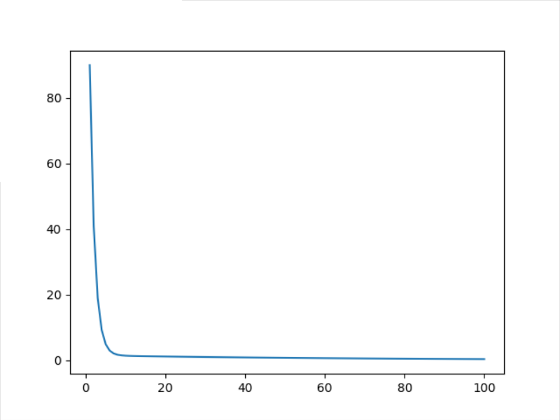
3.2 results of 100 optimizations

Note: y_pred defaults to the value of y when x=4 (i.e. y=8). The closer it is to 8, the better the fitting effect

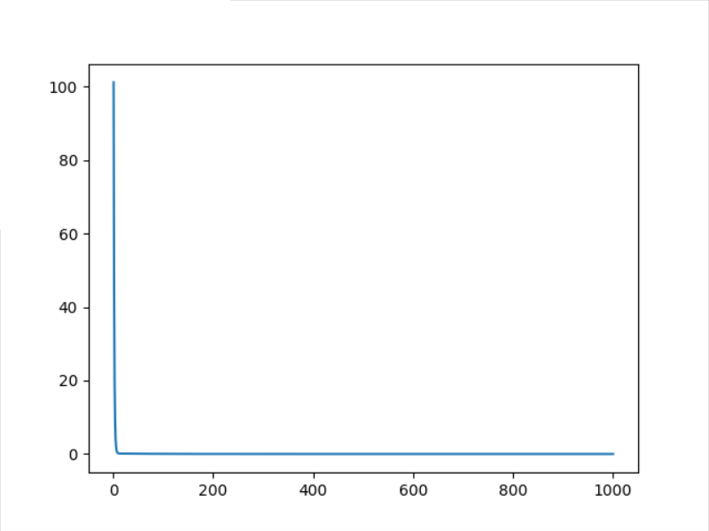
3.3 results of 1000 optimizations

4. Comparison of different optimization methods

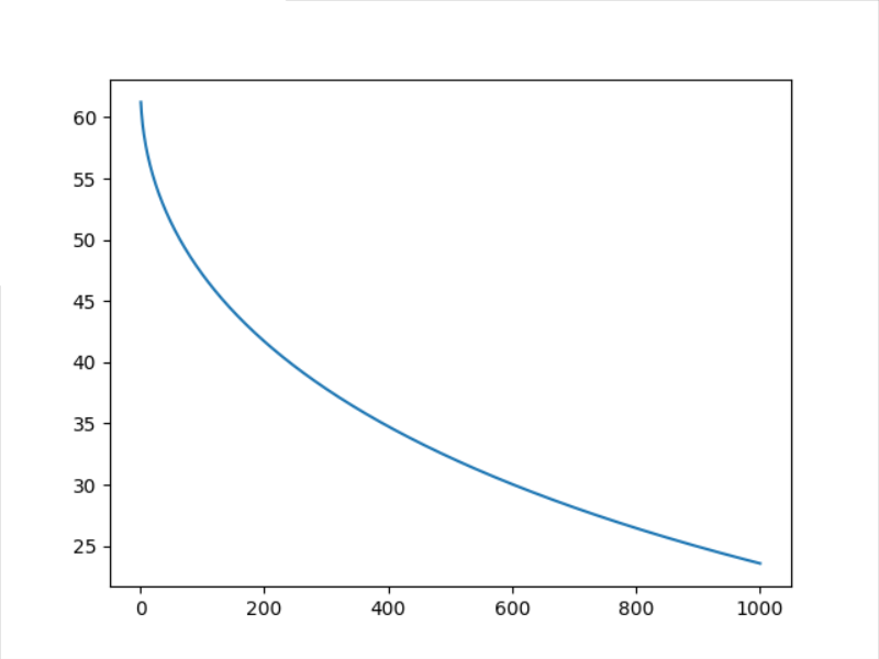
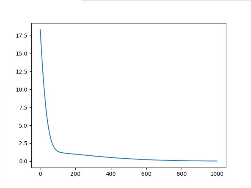
Note: the SGD optimization method has been used previously. Next, several other optimization methods will be used to iterate 1000 times and observe the effect

4.1 Adagrad

4.2 Adam

4.3 Adamax

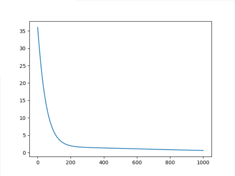
4.4 ASGD

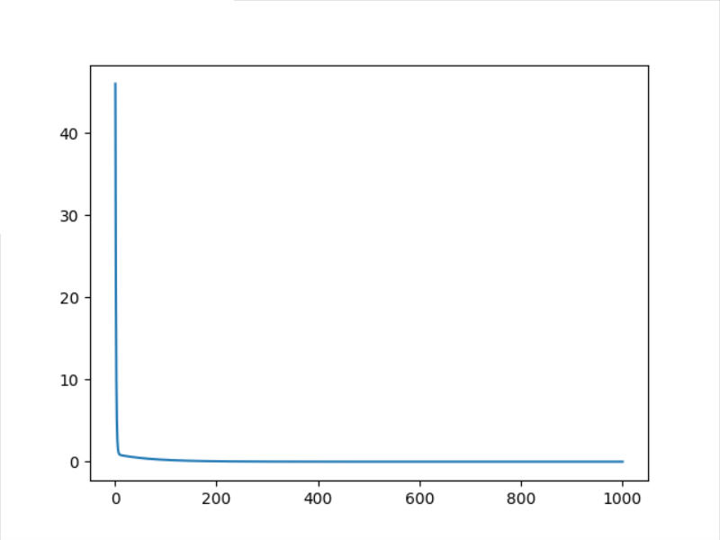
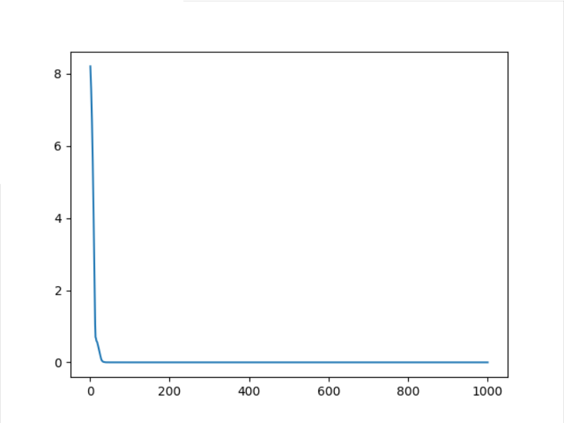
Here, we can see that the speed of asgd decline is quite fast. We only set and adjust it 100 times and observe its decline speed again

ASGD = 100

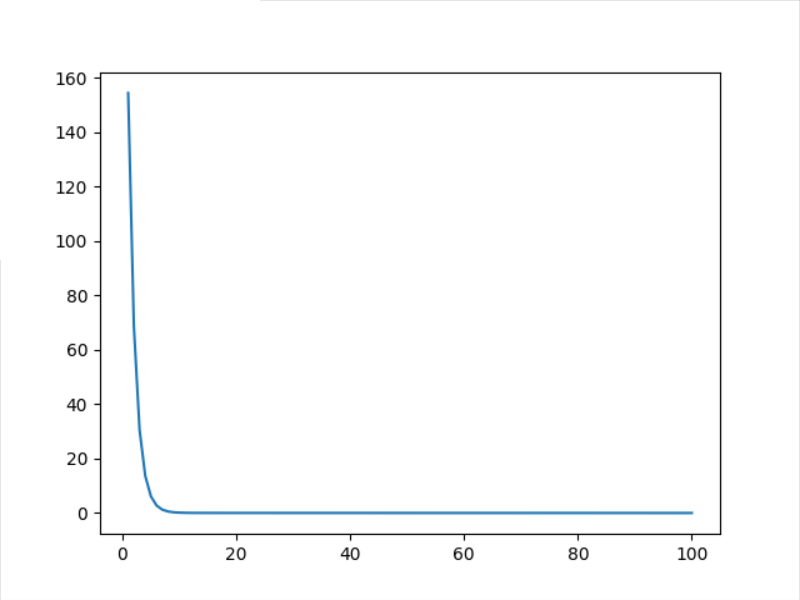
It can be seen that the decline speed of ASGD optimization method is still very fast, and it has been very close to the real value in about 20 iterations

4.5 RMSprop

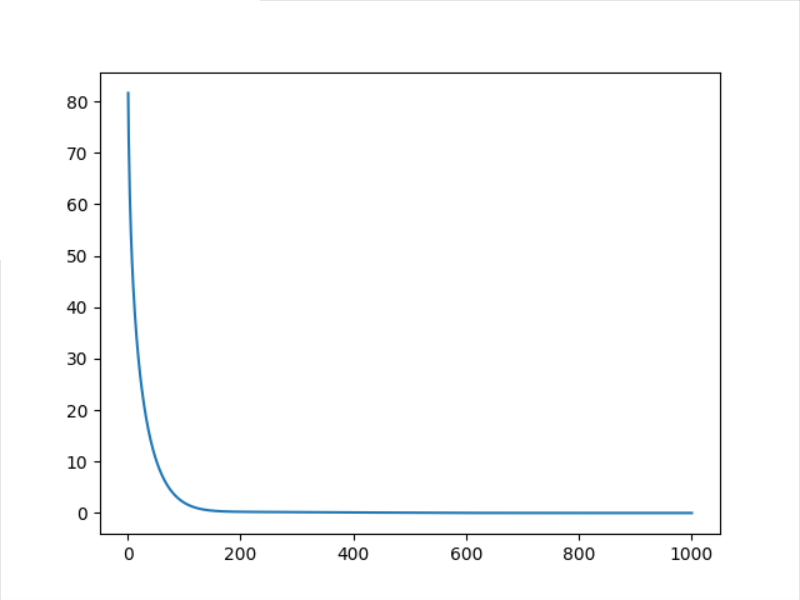
4.6 Rprop

Write at the end

This article is The final collection of PyTorch deep learning practice The solutions of some after-school exercises corresponding to the course are only for your reference

Ladies and gentlemen, I've seen it here. Please use your fingers to praise the blogger 8. Your support is the author's greatest creative power (＾－＾)＞
Lack of talent and learning. If there is any mistake, please correct it
This article is only for the purpose of learning and communication, not for any commercial purpose. If copyright issues are involved, please contact the author as soon as possible