1, Introduction to cellular automata

Development of cellular automata
The original cellular automata was proposed by von Neumann in the 1950s to simulate the self replication of biological cells However, it has not been valued by the academic community
In 1970, after John Horton Conway of Cambridge University designed a computer game "life game", cellular automata attracted the attention of scientists

In 1983, S.Wolfram published a series of papers The models generated by 256 rules of elementary cellular machines are deeply studied, and their evolution behavior is described by entropy. Cellular automata are divided into stationary type, periodic type, chaotic type and complex type

2. Preliminary understanding of cellular automata
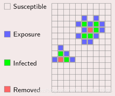
Cellular automata (CA) is a method used to simulate local rules and local connections. A typical cellular automata is defined on a grid. The grid at each point represents a cell and a finite state. Change rules apply to each cell and run simultaneously. Typical change rules depend on the state of the cell and its state (4 or 8) the status of neighbors.

The change rule of 3-cell & cell state
Typical change rules depend on the state of the cell and the state of its (4 or 8) neighbors.

Application of 4-cellular automata
Cellular automata has been applied to physical simulation, biological simulation and other fields.

matlab programming of 5-cell cellular automata
Combined with the above, we can understand that cellular automata simulation needs to understand three points. One is cell. In matlab, it can be understood as a square block composed of one or more points in the matrix. Generally, we use a point in the matrix to represent a cell. The second is the change rule, which determines the state of the cell at the next moment. The third is the state of cells. The state of cells is user-defined and usually opposite, such as the living state or death state of organisms, red light or green light, obstacles or no obstacles at this point, etc.

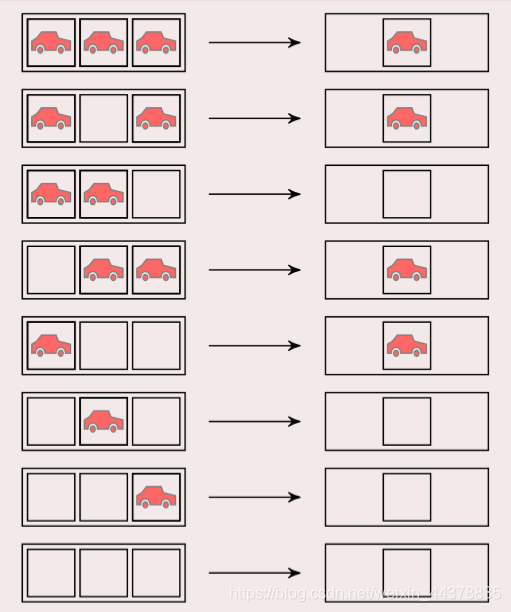
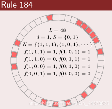
6 one dimensional cellular automata -- traffic rules
definition:
6.1 cells are distributed on one-dimensional linear grid
6.2 cells have only two states: car and empty

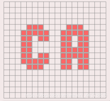
7 two dimensional cellular automata -- life game
definition:
7.1 cells are distributed on two-dimensional square grid
7.2 cells have only two states of life and death

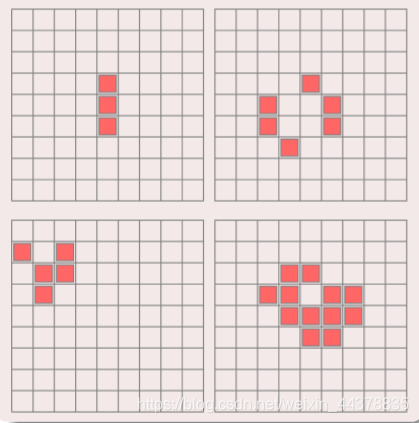
The cellular state is determined by the surrounding eight neighbors
Rules:

Skeleton: death; Smiling face: survival
If there are three smiling faces around, the middle becomes a smiling face
Less than two smiling faces or more than three, the middle becomes death.

8 what is cellular automata
Discrete system: cell is defined in finite time and space, and the state of cell is finite
Dynamic system: the behavior of cellular automata has dynamic characteristics
Simplicity and complexity: cellular automata uses simple rules to control interacting cells to simulate a complex world

9 constituent elements

(1) Cell

Cell is the basic unit of cellular automata:
State: each cell has the function of memory storage state
Discrete: in simple cases, there are only two possible states of cells; In complex cases, cells have many states
Update: the state of the cell is constantly updated according to the dynamic rules
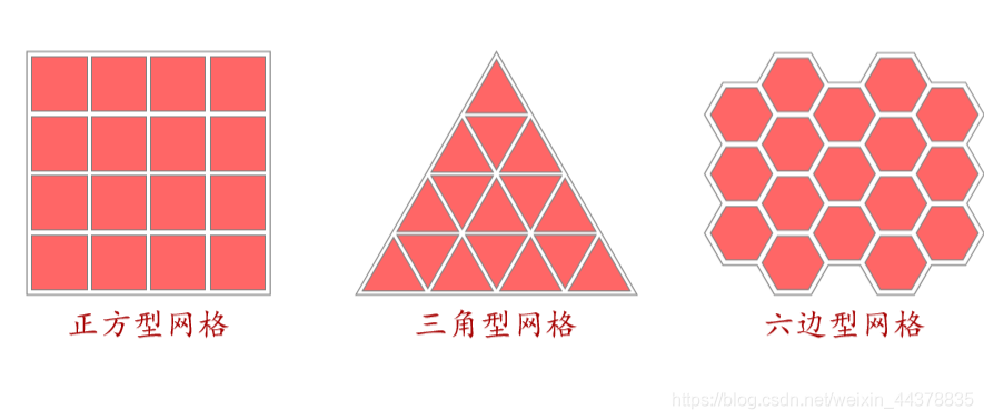
(2) Mesh (Lattice)
Different dimensional grid

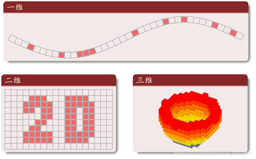
Common 2D mesh

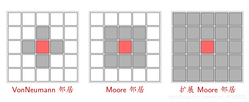
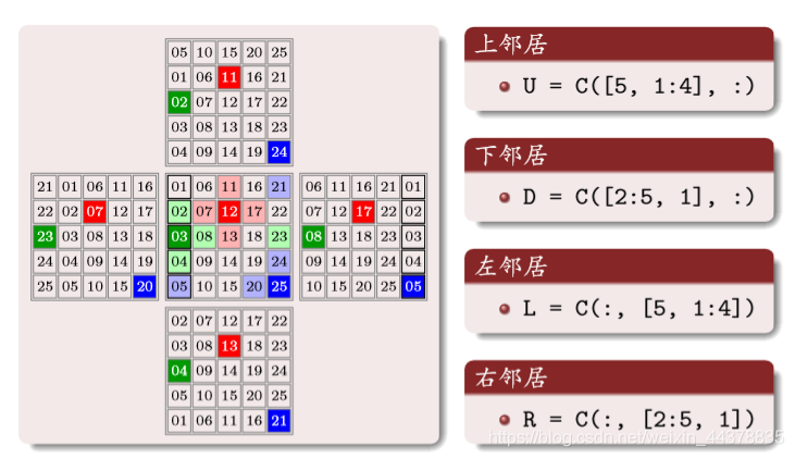
(3) Neighbors

(4) Boundary

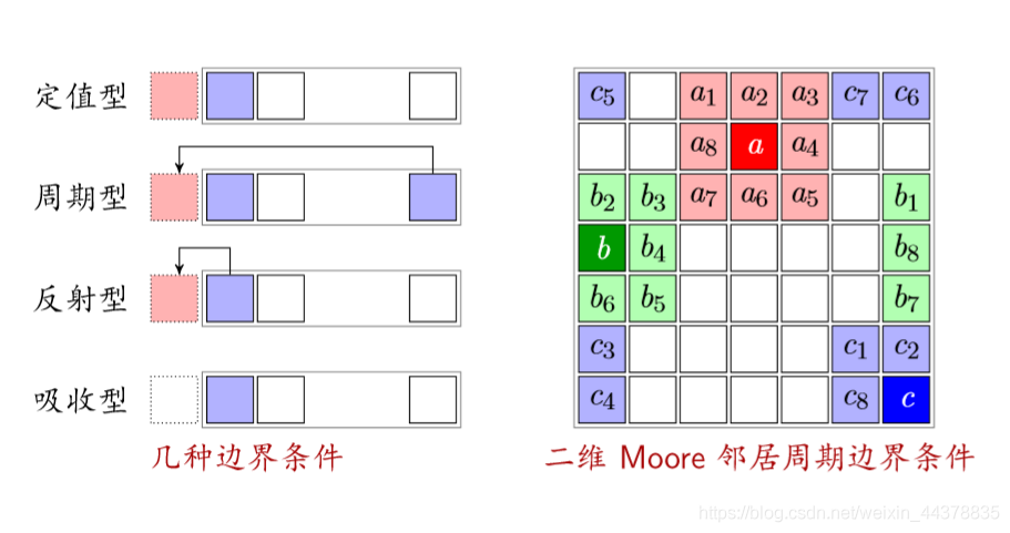
Reflective: a state with itself as a boundary
Absorption type: regardless of the boundary (the car disappears when it reaches the boundary)

(5) Rule (state transition function)
Definition: determine the dynamic function of the cell state at the next time according to the current state of the cell and its neighbors. In short, it is a state transition function
Classification:
Summation: the state of a cell depends on and only depends on the current state of all its neighbors and its own current state
Legal type: sum type rules are legal type rules However, if the rules of cellular automata are limited to summation, cellular automata will have limitations
(6) Forest fire

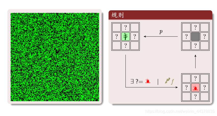
Green: trees; Red: fire; Black: open space.
Three state cycle transitions:
Tree: when there is fire around or struck by lightning, it becomes fire.
Open space: change into trees with probability p
Rational analysis: red is fire; Ash is open space; Green is a tree

The density sum of the three states of the cell is 1

The density of fire into open space is equal to the density of open space into trees (newly grown trees are equal to burned trees)

f is the probability of lightning: far less than the probability of tree generation; T s m a x T_{smax}T smax
It's a time scale for a large group of trees to be burned
Program implementation
Periodic boundary conditions
Buy

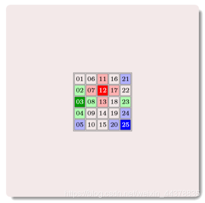
The number is number
Building neighbor matrix

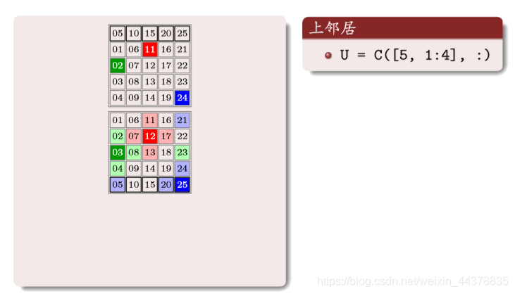
The number in the above matrix corresponds to the upper neighbor number of the same position number of the original matrix, one by one
Similarly:

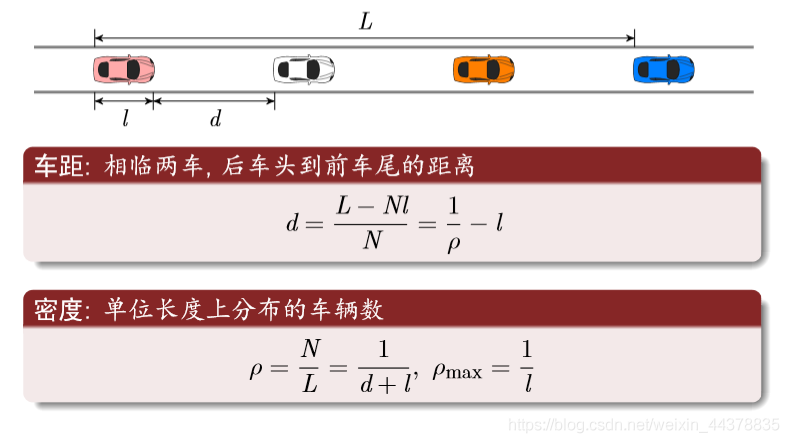
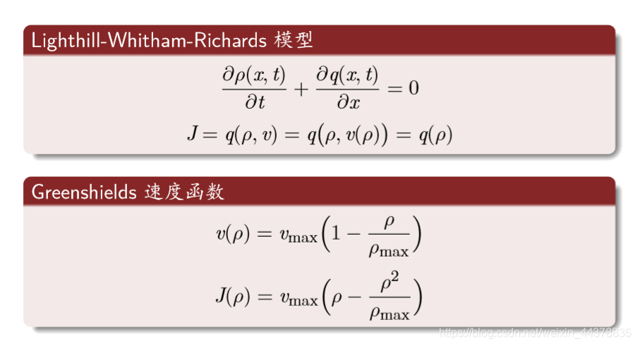
(7) Traffic concept
Distance and density

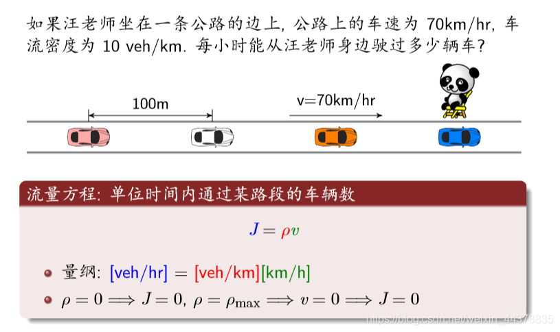
Flow equation

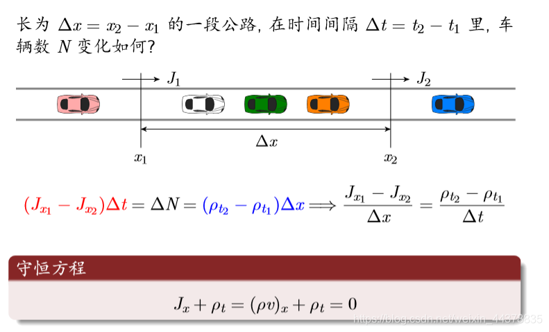
conservation equation

Spatiotemporal trajectory (horizontal axis is space and vertical axis is time)

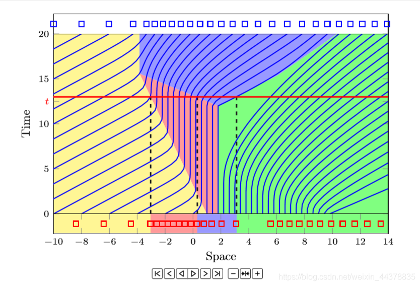
The intersection of the red line and the blue line indicates the location of each time car.
If it is a vertical line, it indicates the corresponding time of the vehicle in this position

Macro continuous model:

Most common rules:

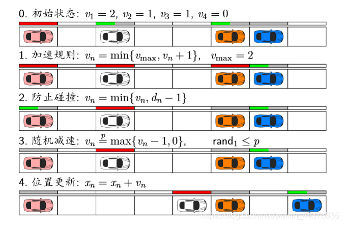
The red bar indicates that the speed is full.

1 acceleration rule: no more than v m a x (2 grids / s) v#{max} (2 grids / s) V
max (2 grids / s)
2. Collision prevention: do not exceed the vehicle distance

Theoretical analysis:

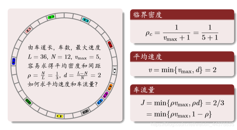
Result analysis: density and flow

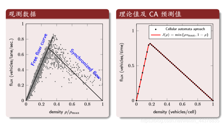
The first figure: the abscissa is the normalized density, and the ordinate is the traffic flow. The second figure: theoretical values and CA results

Result analysis: spatiotemporal trajectory

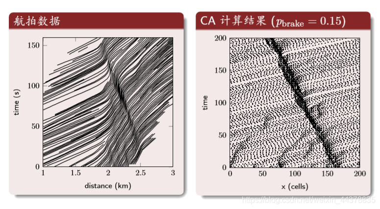
The dark area in the middle is the area of traffic jam.

2, Partial source code

% take TheSeed The obstacles and doors in the model room were fixed and divided into several small rooms, and the rest remained unchanged
% calculates static field - returns computed static field
% input:
% n - x dimension
% m - y dimension
% doors - array of doors - each row represents one door cell and consist of two columns - (i,j) coords
% doorLengths - array, containd lengths of each door
% contraction - effective DoorLength/doorLength
% nObstacles - number of obstacles. Necassary, because matlab don't know how to pass array with zero length
% Ks - influence for door field
% Kw - influence of wall field
% pI - Inertia factor=exp(kI)，kI Is the sensitivity factor.
% pW - wall potential，Avoid approaching obstacles and walls when people move

function main()

GridDims=[50,50];                % Set room size because one unit is 0.5m，So this represents 11 m*5m The size of the room, a wall also occupies a unit
population=500;                   % Set number of people



nDoors=1;                        % This parameter is no longer used in this model
doorLengths=[6];


% nObstacles=5;                    % I also want to see if the settings of these two lines need to be kept


Ks=1000;
Kw=3;

alpha=0.8;
delta=0.8;
miu=0.1;

contraction=0.6;                 % This thing.. It is used to express the contraction of the wide outlet, and I don't understand the function of this

% paramsDoors=[nDoors,lengths];
[Occupied,Doors,Obstacles]=populate(population,GridDims);
params=[Ks,Kd,alpha,delta,miu,Ki];

% StatField=ones(GridDims(1),GridDims(2));    % alerady in exponenta
% What's the use of the line above? stay calcStatField In the function, shilling is 0 again

DynField=zeros(GridDims(1),GridDims(2));

if(Ks)
    StatField=calcStatField(GridDims, Doors, doorLengths, contraction, Obstacles, Ks, Kw);     % The Seed Version, without too many modifications
%     StatField=myCalcStatField(GridDims,Occupied,Doors,lengths,contraction,nObstacles,population,Ks, Kw);
end

%movie object to record
mov=VideoWriter('output.avi');   
open(mov);



cnt = 0;
evacuated = 0;
while( (evacuated ~= population))
cnt = cnt + 1;
draw(Occupied);
F = getframe(fig);
writeVideo(mov,F);
pause(0.1)                                % Pause interval of each step
[Occupied, DynField, cur_evacuated] = myUpdate(Occupied, DynField, StatField, params);
evacuated = evacuated + cur_evacuated;
end

draw(Occupied);

close(mov);
disp(cnt);                                 % time
end
% calculation S Field, this is based on The Seed，Basically unchanged version
% stay The Seed Inside, on the surface Doors Defined as nDoors A matrix with two rows and two columns, actually Doors Is a matrix with two rows and two columns in width.
% For example, if there is only one transverse door with a width of 7, then Doors Is a matrix with 7 rows and 2 columns, and each row corresponds to one of the doors cell. 
function StatField = calcStatField(GridDims, Doors, doorLengths, contraction, obstacles, Ks, Kw)

n = GridDims(1);
m = GridDims(2);
nDoors = size(doorLengths);

% if nObstacles ~= 0                             % What are these three lines for? I commented out that they can run the same program.
% nObstacles = size(obstacles);                  % My definition of obstacles here is not so simple, so I think I may need to make some changes
% end

StatField = zeros(n, m);                       % Initialize to 50*50 0 matrix of
maxDist = 0;

for i = 2: n-1
for j = 2: m-1
minDist = inf;                                 % inf Is infinite
% Find the shortest path to the exit

cnt = 1;
for k = 1: nDoors

% I don't understand these two steps. What is the effective width? What basis?
effectiveLength = contraction*doorLengths(k);                  % Effective width  contraction = 0.6  doorLengths Value range of[5,10]
offset = floor((doorLengths(k)-effectiveLength) * 0.5);       % floor(x)Yes, make it less than or equal to x The maximum integer of. offset Value range of[1,2].

% this for To find this(i,j)The closest distance to the corresponding door.
for l = offset: offset + effectiveLength-1                    % In this place l It's lowercase L!It doesn't matter if there are decimals. When you cycle, you take an integer.

% power(a,b)yes a Of each element in the b Power. po express(i,j)The square of the distance to the door.
po = power((i-Doors(cnt+l, 1)),2)+power((j-Doors(cnt+l,2)), 2);  % doors(cnt+l,1)It's the door i Coordinates, doors(cnt+l,2)It's the door j coordinate
% (This place is lowercase L，Not 1) cnt+l Because: what is calculated here is(i,j)How many squares are there between the door and the door, so+l.

% If the door is not visible, its distance is greater than the straight line, so it exceeds minDist
if(po >= minDist)                                             % The purpose is to find the smallest Dist
continue;
end

% check if there is visible path to doors
% TODO:

minDist = po;                                                 % So it's not infinite
end
cnt = cnt + doorLengths(k);
end

StatField(i, j) = minDist;
if(maxDist < minDist)
maxDist = minDist;                                              % Find the furthest distance from the door in the whole room
end
end
end
dMax = 4;        % Influence radius of wall

StatField(1,:) = -1;       %Whatever's here
StatField(n,:) = -1;
StatField(:,1) = -1;
StatField(:,m) = -1;

for i = 2: n-1
for j = 2: m-1
    %The attraction of the door
    %if(maxDist == StatField(i,j))
%StatField(i,j) = 0;
%else             %exp(Ks/(1-sqrt(maxDist/StatField(i,j)))); 
StatField(i,j) = Ks*exp(-StatField(i,j)/maxDist*750);
%end     The distance above is actually squared. I still need to check whether I need to square it back
% find min dist to the obstacle 
minDistObst = inf; 
nObstacles = 0; 
for l = 1: nObstacles 
    po = power((i-obstacles(l, 1)),2)+power((j-obstacles(l,2)), 2); 
    if(po < minDistObst) 
        minDistObst = po; 
    end 
end 
%StatField(i,j) = 1;      % for visualization of repulsive wall field 
% repulsive potential of walls 
if(minDistObst ~= inf) 
    if(minDistObst == 0) 
        StatField(i,j) = 0; 
        continue; 
    end

minDistObst = sqrt(minDistObst); 
if(minDistObst < dMax) 
    StatField(i,j) = StatField(i,j)*exp(Kw*(1-(dMax/minDistObst))); 
end
end
end
end
end

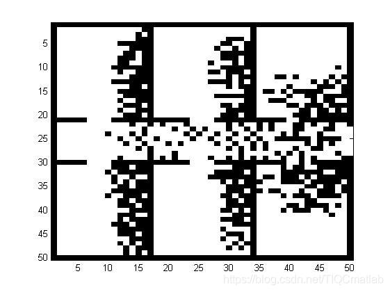
3, Operation results

4, matlab version and references

1 matlab version
2014a

2 references
[1] Steamed stuffed bun Yang, Yu Jizhou, Yang Shan Intelligent optimization algorithm and its MATLAB example (2nd Edition) [M]. Electronic Industry Press, 2016
[2] Zhang Yan, Wu Shuigen MATLAB optimization algorithm source code [M] Tsinghua University Press, 2017
[3][mathematical modeling] cellular automata. Blogger: binary artificial intelligence