This article is the original article of CSDN blogger "hanging small", and the reprint has been approved by the original blogger.
Original link: https://blog.csdn.net/m0_46988935/article/details/109234900
catalogue
4, Traditional lane line detection process
preface
Common lane line detection methods can be roughly divided into three categories:
- traditional method
The lane line features are extracted from the image taken by the camera by using the traditional image processing base. - The combination of traditional image processing and deep learning
The feature information extracted by deep learning can not be used directly. The traditional image processing method is used to cluster and fit the line feature points. - End to end deep learning method
Learn lane line features directly from the input image without complex preprocessing, manual feature extraction and post-processing. Combined with various geometric prior knowledge of lane line, design loss function supervision network training to improve the robustness and accuracy of lane line detection.
This paper mainly introduces how to realize a simple traditional lane line detection project, expounds the process of traditional lane line detection in detail, and summarizes the idea of Hough transform and canny edge detection process.
1, What is Hough transform
Hough transform is a kind of feature detection, which is widely used in image analysis, computer vision and digital image processing. The classical Hough transform is to detect the straight lines in the picture. After that, Hough transform can not only recognize the straight lines, but also any shape, such as circles and ellipses.
Problem: for humans, it is very easy to recognize a straight line or circle in an image. But for the computer, what an image presents is only a matrix with gray value from 0 to 255. It can't judge which lines in the matrix are straight lines and which are not. Hough change is an algorithm to help the computer "see" the straight lines or circles in the image.
1. Basic ideas
The traditional image is changed from the x-axis and y-axis coordinate system to the parameter space (m, b) or hough space, and the local maximum value is calculated through the parameter space (which can be called accumulation space), so as to determine the position of a line or circle in the original image.
2. Common Hough transform
- Hough transform based on Cartesian coordinate system space
In the plane rectangular coordinate system, a straight line is determined by its slope m0 and intercept b0. In other words, the points on a straight line use the same pair of m0 and b0. Therefore, if there is a coordinate system that forms a parameter space with (m0, b0) as the parameter from m0 as the horizontal axis and b0 as the vertical axis, the point on a straight line in the plane rectangular coordinate system can be expressed as a point in the parameter space.
When any point in the plane rectangular coordinate system changes with m0 and b0, what appears in the parameter space is A straight line. Take any two points A and B in the plane rectangular coordinate system and project them in the parameter space. The two straight lines intersect at A point C(p,q). The information reflected in intersection C is that the slope of the straight line connecting points A and B is p and the intercept is Q. Therefore, we can understand that Hough transform is actually to calculate the value of the accumulated point in the parameter space. The larger the value, the higher the confidence of the line represented by the parameters m0 and b0 of the point.
However, when the straight line is perpendicular to the X-axis, the slope m0 will become infinite, which will cause the phenomenon that it can not be carried out in computer numerical operation. Therefore, a Hough transform based on polar coordinate space is proposed to solve this problem.
- Hough transform based on polar coordinate space
Polar coordinate is a coordinate system composed of pole, polar axis and polar diameter. Then, a straight line can be uniquely determined by the vertical distance from the origin to the straight line and the angle between the vertical line and the X axis. Projection to the parameter space can be expressed as a sinusoidal curve. Then the polar coordinate system parameter space is similar to the Cartesian coordinate system parameter space, which can be regarded as an accumulation space to calculate the local maximum and predict the straight line.
However, in the real application scenario, many straight lines are not very fine, and there are more or less deviations, resulting in that the curves in the parameter space cannot intersect at an accurate point. Therefore, we need to divide the parameter space into blocks, and the step size of the blocks is the polar diameter and polar angle per unit length. Secondly, calculate the accumulated number of intersections in the unit area, recognize the area value greater than the threshold as a straight line, and store its parameters.
However, the block step size will also have an impact on the detection accuracy. If the score is too small, the calculation cost will rise, and if the score is too large, the calculation accuracy will decline. The application of real scene will use a Mask method to extract the region of interest, so as to greatly reduce the amount of calculation.
2, Edge detection algorithm
Edge detection algorithm is essentially a filtering algorithm. The difference lies in the selection of filter, which is consistent with the filtering rules. In order to understand the edge detection operator, we introduce the concept of gradient. Gradient can be understood as the change speed of pixel gray value in the field of digital image processing, but in digital image processing, the practical application does not need derivation, only simple addition and subtraction.
Several basic edge detection filters: sobel, prewitt and roberts operators.
Problem: there are many problems in the edge map obtained by directly using the basic edge operator, such as noise pollution is not eliminated, the edge line is too thick and wide, etc. Therefore, we introduce an advanced edge detection operator - canny operator.
The specific steps of the popular canny algorithm:
1. Gaussian filtering
Principle of Gaussian filtering: weighted average according to the gray value of the pixel to be filtered and its neighborhood points according to the parameter rules generated by Gaussian formula.
2. Calculate gradient image and angle image
The gradient detection operator used in canny is the filter obtained by gradient calculation using Gaussian filter. The result is also similar to sobel operator, that is, the closer the pixel is to the center point, the greater the weight is.
The calculation of angle image is relatively simple, and its function provides guidance for the direction of non maximum suppression.
3. Non maximum suppression of gradient image
The gradient image obtained in the previous step has many problems, such as rough edge width, weak edge interference and so on. Now you can use non maximum suppression to find the local maximum value of pixel points, set the gray value corresponding to the non maximum value to 0 and the maximum value point to 1, so you can eliminate most of the non edge pixels. Therefore, the final generated image should be a binary image, Edges are ideally single pixel edges.
4. Use double threshold for edge connection
The edge quality obtained through the above three steps has been very high, but there are still many false edges. Therefore, the algorithm adopted by canny algorithm is the double threshold method. The specific idea is: select two thresholds, set the points less than the low threshold as false edges, and set the points greater than the high threshold as strong edges. The pixels in the middle need further inspection.
3, Experimental environment
Pycharm2018.2.4 x64 + opencv2.4.10
4, Traditional lane line detection process
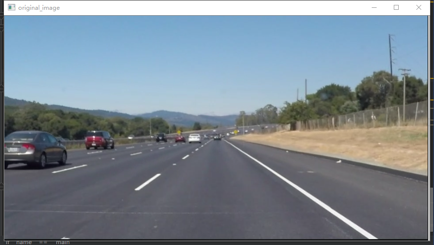
1. Convert color image into gray image
Convert a color image to a gray scale image, that is, from a three channel RGB image to a single channel image.
We need to use CV in opencv Library in this step Cvtcolor function, which realizes color space conversion. Two parameters are required: src - input picture and code - color conversion code. The specific codes are as follows:
#Gray image conversion
def grayscale(image):
    return cv.cvtColor(image, cv.COLOR_RGB2GRAY)
Original drawing:
Grayscale rendering:
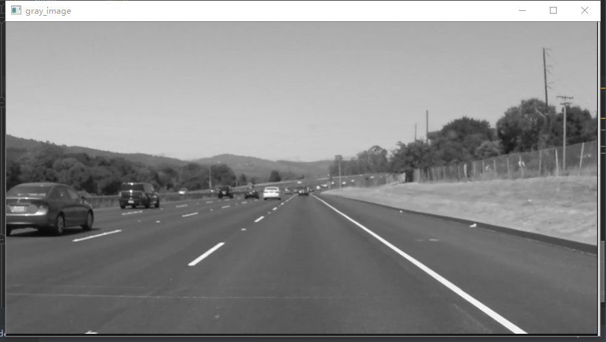
- Why do we need to grayscale color images?
After graying, the color information is lost, many simple recognition algorithms do not rely on color, and the color itself is very vulnerable to illumination and other factors. The key and essential part of object recognition is to calculate the gradient. Color itself is difficult to provide key information. Only the information in gray image is enough. After graying, the matrix is simplified and the operation speed is improved.
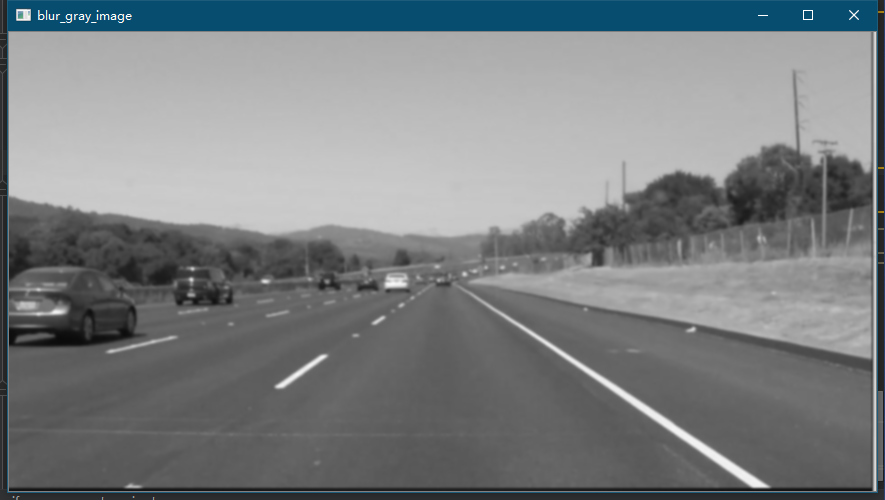
2. Gaussian filtering
Gaussian filtering algorithm is a common way to remove high-frequency noise. Generally speaking, Gaussian filtering is the process of weighted average of the whole image. The value of each pixel is obtained by weighted average of itself and other pixel values in the neighborhood. The principle of Gaussian filtering is to weighted average the gray values of the pixels to be filtered and their neighborhood points according to the parameter rules generated by Gaussian formula.
We need to use CV in opencv Library in this step Gaussian blur function, where the parameters used are: src -- input image, kernel_size - the size of Gaussian kernel, sigma - Gaussian standard deviation (generally 0 by default). The specific code is as follows:
# Gaussian filtering
def gaussian_blur(image, kernel_size):
	return cv.GaussianBlur(image, (kernel_size, kernel_size), 0)
Rendering after Gaussian filtering:
- Compare the four filtering methods
Mean filter, Gaussian filter, median filter, bilateral filter - Two purposes of filtering
The image features are extracted by filtering, and the information carried by the image is simplified as other subsequent image processing.
In order to meet the needs of image processing, the noise mixed in image digitization is eliminated by filtering.
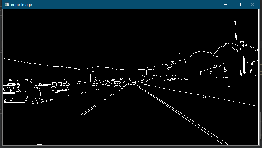
3. Canny edge detection
We need to use CV in opencv Library in this step Canny function, where the parameters used are: src -- input image, low_threshold -- low threshold, high_threshold - high threshold, the specific code is as follows:
# Canny edge detection
def canny(image, low_threshold, high_threshold):
   	 return cv.Canny(image, low_threshold, high_threshold)
Effect drawing after Canny edge detection:
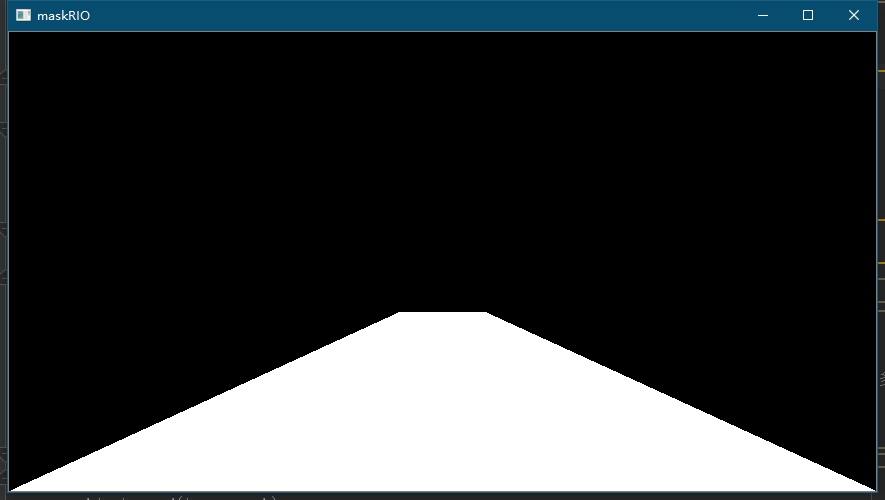
4. Generate Mask and extract ROI
The Mask is used to reduce the computational cost, that is, the algorithm is calculated only in the part we are interested in. The design idea is as follows:
- Generate a mask matrix consistent with the size dimension of the original image and initialize it to all 0, that is, all black.
- Build the region of interest on the mask according to the original image
- Using cv. In opencv The fillpoly() function fills the defined polygon contour with 1, that is, all white
- Using cv. In opencv Bitwise() function and canny edge detect the image by bit and, retain the white pixel value in the corresponding region of interest in the original image, and eliminate the black pixel value
The region of interest designed here is roughly estimated to determine the coordinates of four vertices, and the graph is trapezoid.
 The specific implementation code is as follows:
# Generate the region of interest, i.e. Mask
def region_of_interest(image, vertices):
mask = np.zeros_like(image) # Generate zeros moments with consistent image size
# Fills the middle region of vertex vertices
if len(image.shape) > 2:
channel_count = image.shape[2]
ignore_mask_color = (255,) * channel_count
else:
ignore_mask_color = 255
# Filling function
cv.fillPoly(mask, vertices, ignore_mask_color)
masked_image = cv.bitwise_and(image, mask)
return masked_image
# Generate Mask
vertices = np.array([[(0, imshape[0]), (9 * imshape[1] / 20, 11 * imshape[0] / 18),
(11 * imshape[1] / 20, 11 * imshape[0] / 18), (imshape[1], imshape[0])]], dtype=np.int32)
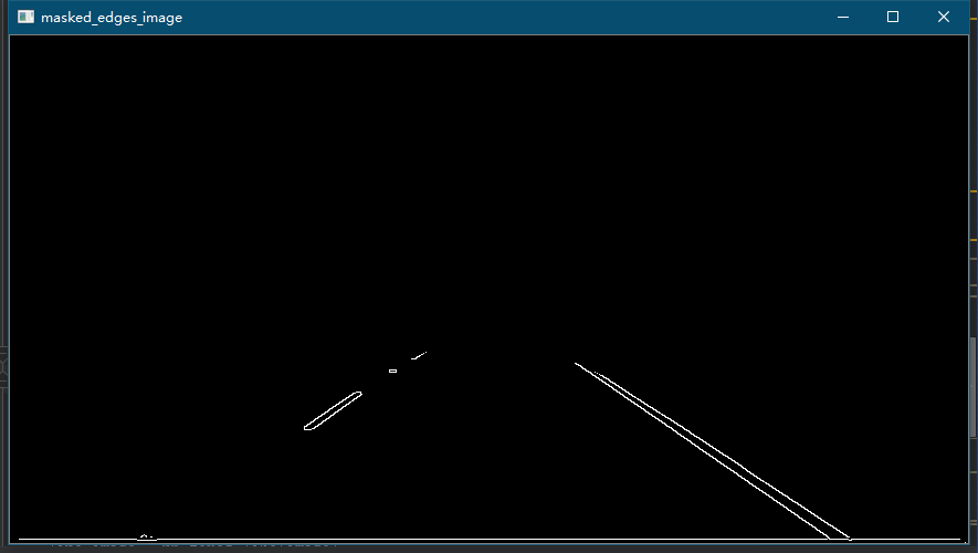
masked_edges = region_of_interest(edge_image, vertices)
After bitwise and of the image after the region of interest and canny edge detection, the resulting effect image is as follows:
5. Line detection based on Hough transform
The Opencv encapsulated function CV is used Houghlinesp function uses the following parameters:
- Image: input image, usually the image after canny edge detection processing
- rho: distance precision of line segments in pixels
- theta: angular accuracy of pixels in radians (np.pi/180 is more appropriate)
- Threshold: threshold of Hough plane accumulation
- minLineLength: minimum length of line segment (pixel level)
- maxLineGap: maximum allowable breaking length
The specific codes are as follows:
def hough_lines(img, rho, theta, threshold, min_line_len, max_line_gap):

    # rho: distance precision of line segments in pixels
    # theta: angular accuracy of pixels in radians (np.pi/180 is more appropriate)
    # Threshold: threshold of Hough plane accumulation
    # minLineLength: minimum length of line segment (pixel level)
    # maxLineGap: maximum allowable breaking length
    lines = cv.HoughLinesP(img, rho, theta, threshold, np.array([]), minLineLength=min_line_len, maxLineGap=max_line_gap)
    return lines
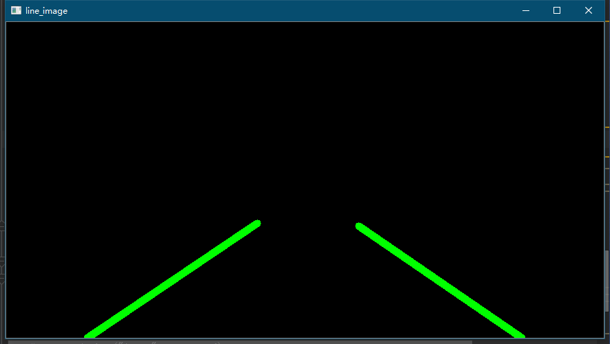
6. Draw lane lines
This step is to draw the line detected in the previous step, but it will be found that the line directly drawn after Hough transform can see that multiple line segments are adjacent to each other, and what we expect is single lane line detection. In order to intuitively experience and follow-up processing, it is necessary to further preprocess the straight line detected in the previous step. The specific processing methods are as follows:
- Calculate the slope of each straight line and classify it into the left and right lists respectively
- Calculate the average value m0 of the slope and the highest point A of the obtained list
- According to the average slope m_{0}, highest point calculation line segment, intersection B coordinate below the image
- Connect the highest point A and intersection B
The specific codes are as follows:
line_image = np.zeros_like(image)
def draw_lines(image, lines, color=[255,0,0], thickness=2):

    right_y_set = []
    right_x_set = []
    right_slope_set = []

    left_y_set = []
    left_x_set = []
    left_slope_set = []

    slope_min = .35  # Slope low threshold
    slope_max = .85  # Slope high threshold
    middle_x = image.shape[1] / 2  # x coordinate of image center line
    max_y = image.shape[0]  # Maximum y coordinate

    for line in lines:
        for x1, y1, x2, y2 in line:
            fit = np.polyfit((x1, x2), (y1, y2), 1)    # Quasi synthetic line
            slope = fit[0]  # Slope

            if slope_min < np.absolute(slope) <= slope_max:

                # Save the point where the slope is greater than 0 and the X coordinate of the line segment is on the right of the center line of the image as the right lane line
                if slope > 0 and x1 > middle_x and x2 > middle_x:
                    right_y_set.append(y1)
                    right_y_set.append(y2)
                    right_x_set.append(x1)
                    right_x_set.append(x2)
                    right_slope_set.append(slope)

                # Save the point whose slope is less than 0 and the X coordinate of the line segment is on the left of the center line of the image as the left lane line
                elif slope < 0 and x1 < middle_x and x2 < middle_x:
                    left_y_set.append(y1)
                    left_y_set.append(y2)
                    left_x_set.append(x1)
                    left_x_set.append(x2)
                    left_slope_set.append(slope)

    # Draw left lane line
    if left_y_set:
        lindex = left_y_set.index(min(left_y_set))  # the peak
        left_x_top = left_x_set[lindex]
        left_y_top = left_y_set[lindex]
        lslope = np.median(left_slope_set)   # Calculate average

    # Calculate the intersection between the lane line and the lower part of the picture according to the slope as the starting point
    left_x_bottom = int(left_x_top + (max_y - left_y_top) / lslope)

    # Draw line segments
    cv.line(image, (left_x_bottom, max_y), (left_x_top, left_y_top), color, thickness)

    # Draw the right lane line
    if right_y_set:
        rindex = right_y_set.index(min(right_y_set))  # the peak
        right_x_top = right_x_set[rindex]
        right_y_top = right_y_set[rindex]
        rslope = np.median(right_slope_set)

    # Calculate the intersection between the lane line and the lower part of the picture according to the slope as the starting point
    right_x_bottom = int(right_x_top + (max_y - right_y_top) / rslope)

    # Draw line segments
    cv.line(image, (right_x_top, right_y_top), (right_x_bottom, max_y), color, thickness)
The effect drawing of lane line is as follows:
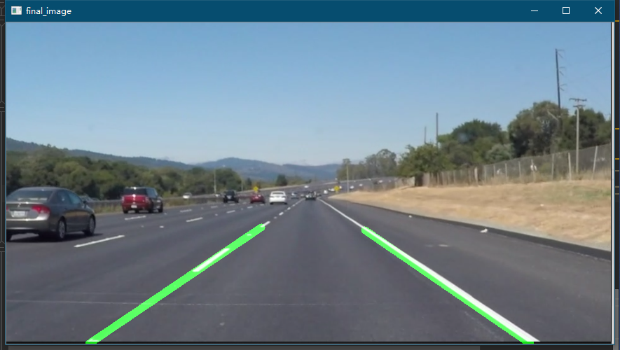
7. Image fusion
This step is to fuse the original color image with the lane line image we just drew. Here we need to introduce a function cv Addweighted, parameter src1 -- original image or matrix; alpha -- the weight corresponding to the original image; src2 -- second image; beta -- weight corresponding to the second image; gamma -- added to the value as a whole. The default value is 0.
Here, we set the weight of the original image to 0.8 and the lane line image to 1, then the final effect is that the lane line is more obvious and the visualization degree is improved. The specific code is as follows:
# The original image and lane line image are fused in a:b scale
def weighted_img(img, initial_img, a=0.8, b=1., c=0.):
    return cv.addWeighted(initial_img, a, img, b, c)
The final effect drawing is as follows:
5, Complete code
import numpy as np
import cv2 as cv
import matplotlib.pyplot as plt

# Gray image conversion
def grayscale(image):
    return cv.cvtColor(image, cv.COLOR_RGB2GRAY)

# Canny edge detection
def canny(image, low_threshold, high_threshold):
    return cv.Canny(image, low_threshold, high_threshold)

# Gaussian filtering
def gaussian_blur(image, kernel_size):
    return cv.GaussianBlur(image, (kernel_size, kernel_size), 0)

# Generate the region of interest, i.e. Mask
def region_of_interest(image, vertices):

    mask = np.zeros_like(image)  # Generate zeros moments with consistent image size

    # Fills the middle region of vertex vertices
    if len(image.shape) > 2:
        channel_count = image.shape[2]
        ignore_mask_color = (255,) * channel_count
    else:
        ignore_mask_color = 255

    # Filling function
    cv.fillPoly(mask, vertices, ignore_mask_color)
    masked_image = cv.bitwise_and(image, mask)
    return masked_image

# The original image and lane line image are fused in a:b scale
def weighted_img(img, initial_img, a=0.8, b=1., c=0.):
    return cv.addWeighted(initial_img, a, img, b, c)

# def reset_global_vars():
#
#     global SET_LFLAG
#     global SET_RFLAG
#     global LAST_LSLOPE
#     global LAST_RSLOPE
#     global LAST_LEFT
#     global LAST_RIGHT
#
#     SET_RFLAG = 0
#     SET_LFLAG = 0
#     LAST_LSLOPE = 0
#     LAST_RSLOPE = 0
#     LAST_RIGHT = [0, 0, 0]
#     LAST_LEFT = [0, 0, 0]

def draw_lines(image, lines, color=[255,0,0], thickness=2):

    right_y_set = []
    right_x_set = []
    right_slope_set = []

    left_y_set = []
    left_x_set = []
    left_slope_set = []

    slope_min = .35  # Slope low threshold
    slope_max = .85  # Slope high threshold
    middle_x = image.shape[1] / 2  # x coordinate of image center line
    max_y = image.shape[0]  # Maximum y coordinate

    for line in lines:
        for x1, y1, x2, y2 in line:
            fit = np.polyfit((x1, x2), (y1, y2), 1)    # Quasi synthetic line
            slope = fit[0]  # Slope

            if slope_min < np.absolute(slope) <= slope_max:

                # Save the point where the slope is greater than 0 and the X coordinate of the line segment is on the right of the center line of the image as the right lane line
                if slope > 0 and x1 > middle_x and x2 > middle_x:
                    right_y_set.append(y1)
                    right_y_set.append(y2)
                    right_x_set.append(x1)
                    right_x_set.append(x2)
                    right_slope_set.append(slope)

                # Save the point whose slope is less than 0 and the X coordinate of the line segment is on the left of the center line of the image as the left lane line
                elif slope < 0 and x1 < middle_x and x2 < middle_x:
                    left_y_set.append(y1)
                    left_y_set.append(y2)
                    left_x_set.append(x1)
                    left_x_set.append(x2)
                    left_slope_set.append(slope)

    # Draw left lane line
    if left_y_set:
        lindex = left_y_set.index(min(left_y_set))  # the peak
        left_x_top = left_x_set[lindex]
        left_y_top = left_y_set[lindex]
        lslope = np.median(left_slope_set)   # Calculate average

    # Calculate the intersection between the lane line and the lower part of the picture according to the slope as the starting point
    left_x_bottom = int(left_x_top + (max_y - left_y_top) / lslope)

    # Draw line segments
    cv.line(image, (left_x_bottom, max_y), (left_x_top, left_y_top), color, thickness)

    # Draw the right lane line
    if right_y_set:
        rindex = right_y_set.index(min(right_y_set))  # the peak
        right_x_top = right_x_set[rindex]
        right_y_top = right_y_set[rindex]
        rslope = np.median(right_slope_set)

    # Calculate the intersection between the lane line and the lower part of the picture according to the slope as the starting point
    right_x_bottom = int(right_x_top + (max_y - right_y_top) / rslope)

    # Draw line segments
    cv.line(image, (right_x_top, right_y_top), (right_x_bottom, max_y), color, thickness)

def hough_lines(img, rho, theta, threshold, min_line_len, max_line_gap):

    # rho: distance precision of line segments in pixels
    # theta: angular accuracy of pixels in radians (np.pi/180 is more appropriate)
    # Threshold: threshold of Hough plane accumulation
    # minLineLength: minimum length of line segment (pixel level)
    # maxLineGap: maximum allowable breaking length
    lines = cv.HoughLinesP(img, rho, theta, threshold, np.array([]), minLineLength=min_line_len, maxLineGap=max_line_gap)
    return lines

def process_image(image):

    rho = 1       # Hough pixel unit
    theta = np.pi / 180    # Hough angle shift step
    hof_threshold = 20   # Hough plane cumulative threshold
    min_line_len = 30    # Minimum length of line segment
    max_line_gap = 60    # Maximum allowable breaking length

    kernel_size = 5      # Gaussian filter size
    canny_low_threshold = 75     # canny edge detection low threshold
    canny_high_threshold = canny_low_threshold * 3    # canny edge detection high threshold

    alpha = 0.8   # Original image weight
    beta = 1.     # Lane line image weight
    lambda_ = 0.

    imshape = image.shape  # Get image size

    # Gray image conversion
    gray = grayscale(image)

    # Gaussian filtering
    blur_gray = gaussian_blur(gray, kernel_size)

    # Canny edge detection
    edge_image = canny(blur_gray, canny_low_threshold, canny_high_threshold)

    # Generate Mask
    vertices = np.array([[(0, imshape[0]), (9 * imshape[1] / 20, 11 * imshape[0] / 18),
                          (11 * imshape[1] / 20, 11 * imshape[0] / 18), (imshape[1], imshape[0])]], dtype=np.int32)
    masked_edges = region_of_interest(edge_image, vertices)

    # Line detection based on Hough transform
    lines = hough_lines(masked_edges, rho, theta, hof_threshold, min_line_len, max_line_gap)
    line_image = np.zeros_like(image)

    # Draw lane line segments
    draw_lines(line_image, lines, thickness=10)

    # Image fusion
    lines_edges = weighted_img(image, line_image, alpha, beta, lambda_)
    return lines_edges

if __name__ == '__main__':
    # cap = cv.VideoCapture("./test_videos/solidYellowLeft.mp4")
    # while(cap.isOpened()):
    #     _, frame = cap.read()
    #     processed = process_image(frame)
    #     cv.imshow("image", processed)
    #     cv.waitKey(1)


    image = cv.imread('./test_images/solidYellowCurve2.jpg')
    line_image = process_image(image)
    cv.imshow('image',line_image)
    cv.waitKey(0)