Firstly, this paper analyzes the process of deep learning, abstracts the key components in neural network, and determines the basic framework; Then code the components in the framework; Finally, based on this framework, an example of MNIST classification is implemented and compared with Tensorflow. If you like this article, please like, collect and pay attention to it.
At present, deep learning frameworks are becoming more and more mature, and the degree of encapsulation is becoming higher and higher for users. The advantage is that these frameworks can be used as tools very quickly, and models can be built and tested with very little code. The disadvantage is that the implementation behind them may be hidden. In this article, the author will design and implement a lightweight (about 200 lines) and easy to expand deep learning framework tinynn (based on Python and Numpy Implementation), hoping to help you understand the basic components of deep learning and the design and implementation of the framework.
Firstly, this paper will analyze the process of deep learning, abstract the key components in neural network and determine the basic framework; Then code the components in the framework; Finally, based on this framework, an example of MNIST classification is implemented and compared with Tensorflow.
catalogue
-
Component abstraction
-
Component implementation
-
Overall structure
-
MNIST example
-
summary
-
appendix
-
reference resources
Component abstraction
First, consider the flow of neural network operation, Neural network operation mainly includes training and prediction (or information) two stages. The basic process of training is: input data - > network layer forward propagation - > calculate loss - > network layer back propagation gradient - > update parameters. The basic process of prediction is input data - > network layer forward propagation - > output results. From the perspective of operation, it can be divided into three types of calculation:
-
Data flow between network layers: forward propagation and back propagation can be regarded as the flow of Tensor tensor (multidimensional array) between network layers (forward propagation flows input and output, and back propagation flows gradient). Each network layer will perform certain operations, and then input the results to the next layer
-
Calculation loss: the intermediate process of connecting forward and back propagation, which defines the difference between the output of the model and the real value, and is used to provide the information required for back propagation
-
Parameter update: a kind of calculation that uses the calculated gradient to update the network parameters
Based on these three types, we can abstract the basic components of the network
-
tensor, which is the basic unit of data in neural network
-
Layer network layer is responsible for receiving the input of the previous layer, performing the operation of this layer and outputting the results to the next layer. Since the flow of tensor has two directions: forward and reverse, we need to implement forward and backward operations for each type of network layer at the same time
-
Loss loss: after the predicted value and real value of the model are given, the component outputs the loss value and the gradient about the last layer (for gradient return)
-
The optimizer optimizer is responsible for updating the parameters of the model using gradients
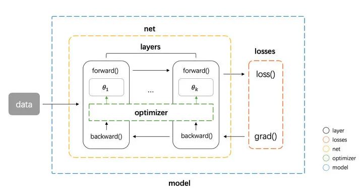
Then we need some components to integrate the above four basic components to form a pipeline
-
net component is responsible for managing the forward and back propagation of tensor between layers, and can provide interfaces for obtaining parameters, setting parameters and obtaining gradients
-
The model component is responsible for integrating all components to form the whole pipeline. That is, the net component propagates forward - > the losses component calculates the loss and gradient - > the net component propagates the gradient back - > the optimizer component updates the gradient to the parameter.
The basic frame diagram is shown in the figure below
Component implementation
According to the above abstraction, we can write the whole process code as follows.
# define model
net = Net([layer1, layer2, ...])
model = Model(net, loss_fn, optimizer)

# training
pred = model.forward(train_X)
loss, grads = model.backward(pred, train_Y)
model.apply_grad(grads)

# inference
test_pred = model.forward(test_X)
First define net. The input of net is multiple network layers, and then pass net, loss and optimizer to the model. The model implements forward, backward and apply_ The three grad interfaces correspond to three functions: forward propagation, back propagation and parameter update. Next, let's look at how to implement each part here.
tensor
Tensor is the basic data unit in neural network. We use numpy directly here The ndarray class is the implementation of the tensor class
numpy.ndarray : https://numpy.org/doc/stable/reference/generated/numpy.ndarray.html
layer
In the above process code, the model performs forward and backward. In fact, the underlying layer is the network layer performing actual operations. Therefore, the network layer needs to provide forward and backward interfaces for corresponding operations. At the same time, the parameters and gradient of this layer should also be recorded. First implement a base class as follows
# layer.py
class Layer(object):
    def __init__(self, name):
        self.name = name
        self.params, self.grads = None, None

    def forward(self, inputs):
        raise NotImplementedError

    def backward(self, grad):
        raise NotImplementedError
The most basic network layer is the fully connected network layer, which is implemented as follows. The forward method receives the input of the upper layer and realizes the operation of the; The backward method receives the gradient from the upper layer, calculates the gradient about the parameter and input, and then returns the gradient about the input. The derivation of these three gradients can be seen in the appendix, and the implementation is given directly here. w_init and b_init is the initializer of parameters and respectively. We use the file initializer in another implementation initializer Py. This part is not the core component, so it will not be introduced here.
# layer.py
class Dense(Layer):
    def __init__(self, num_in, num_out,
                 w_init=XavierUniformInit(),
                 b_init=ZerosInit()):
        super().__init__("Linear")

        self.params = {
            "w": w_init([num_in, num_out]),
            "b": b_init([1, num_out])}

        self.inputs = None

    def forward(self, inputs):
        self.inputs = inputs
        return inputs @ self.params["w"] + self.params["b"]

    def backward(self, grad):
        self.grads["w"] = self.inputs.T @ grad
        self.grads["b"] = np.sum(grad, axis=0)
        return grad @ self.params["w"].T
At the same time, another important part of neural network is activation function. The activation function can be regarded as a network Layer, and the forward and backward methods also need to be implemented. We implement the activation function class by inheriting the Layer class. Here we implement the most commonly used ReLU activation function. func and derivation_func method realizes the forward calculation and gradient calculation of the corresponding activation function respectively.
# layer.py
class Activation(Layer):
    """Base activation layer"""
    def __init__(self, name):
        super().__init__(name)
        self.inputs = None

    def forward(self, inputs):
        self.inputs = inputs
        return self.func(inputs)

    def backward(self, grad):
        return self.derivative_func(self.inputs) * grad

    def func(self, x):
        raise NotImplementedError

    def derivative_func(self, x):
        raise NotImplementedError


class ReLU(Activation):
    """ReLU activation function"""
    def __init__(self):
        super().__init__("ReLU")

    def func(self, x):
        return np.maximum(x, 0.0)

    def derivative_func(self, x):
        return x > 0.0
net
The net class mentioned above is responsible for managing the forward and back propagation of tensor between layers. The forward method is very simple, traversing all layers in order, and the calculated output of each layer is used as the input of the next layer; backward traverses all layers in reverse order and takes the gradient of each layer as the input of the next layer. Here, we also save the gradient of each network layer parameter and return it. Later, we need to update the parameters. In addition, net class also implements the interfaces for obtaining parameters, setting parameters and obtaining gradients, which are also needed for later parameter updates
# net.py
class Net(object):
    def __init__(self, layers):
        self.layers = layers

    def forward(self, inputs):
        for layer in self.layers:
            inputs = layer.forward(inputs)
        return inputs

    def backward(self, grad):
        all_grads = []
        for layer in reversed(self.layers):
            grad = layer.backward(grad)
            all_grads.append(layer.grads)
        return all_grads[::-1]

    def get_params_and_grads(self):
        for layer in self.layers:
            yield layer.params, layer.grads

    def get_parameters(self):
        return [layer.params for layer in self.layers]

    def set_parameters(self, params):
        for i, layer in enumerate(self.layers):
            for key in layer.params.keys():
                layer.params[key] = params[i][key]
losses
We mentioned above that the losses component needs to do two things. Given the predicted value and the real value, we need to calculate the loss value and the gradient about the predicted value. We implement loss and grad methods respectively. Here, we implement the commonly used SoftmaxCrossEntropyLoss loss of multi classification regression. The calculation formulas of loss and gradient grad are derived in the appendix at the end of the paper. The result is directly given here: the loss of cross entropy of multi classification softmax is
The gradient is a little more complex. The calculation formulas of target category and non target category are different. For the target category dimension, its gradient is the output probability of the corresponding dimension model minus one; for the non target category dimension, its gradient is the output probability of the corresponding dimension itself.
The code is implemented as follows
# loss.py
class BaseLoss(object):
    def loss(self, predicted, actual):
        raise NotImplementedError

    def grad(self, predicted, actual):
        raise NotImplementedError


class CrossEntropyLoss(BaseLoss):
    def loss(self, predicted, actual):
        m = predicted.shape[0]
        exps = np.exp(predicted - np.max(predicted, axis=1, keepdims=True))
        p = exps / np.sum(exps, axis=1, keepdims=True)
        nll = -np.log(np.sum(p * actual, axis=1))
        return np.sum(nll) / m

    def grad(self, predicted, actual):
        m = predicted.shape[0]
        grad = np.copy(predicted)
        grad -= actual
        return grad / m
optimizer
Optimizer mainly implements an interface compute_step, this method calculates the step size changed by each parameter when returning to the actual optimization according to the current gradient. Here we implement the commonly used Adam optimizer.
# optimizer.py
class BaseOptimizer(object):
    def __init__(self, lr, weight_decay):
        self.lr = lr
        self.weight_decay = weight_decay

    def compute_step(self, grads, params):
        step = list()
        # flatten all gradients
        flatten_grads = np.concatenate(
            [np.ravel(v) for grad in grads for v in grad.values()])
        # compute step
        flatten_step = self._compute_step(flatten_grads)
        # reshape gradients
        p = 0
        for param in params:
            layer = dict()
            for k, v in param.items():
                block = np.prod(v.shape)
                _step = flatten_step[p:p+block].reshape(v.shape)
                _step -= self.weight_decay * v
                layer[k] = _step
                p += block
            step.append(layer)
        return step

    def _compute_step(self, grad):
        raise NotImplementedError

class Adam(BaseOptimizer):
    def __init__(self, lr=0.001, beta1=0.9, beta2=0.999,
                 eps=1e-8, weight_decay=0.0):
        super().__init__(lr, weight_decay)
        self._b1, self._b2 = beta1, beta2
        self._eps = eps

        self._t = 0
        self._m, self._v = 0, 0

    def _compute_step(self, grad):
        self._t += 1
        self._m = self._b1 * self._m + (1 - self._b1) * grad
        self._v = self._b2 * self._v + (1 - self._b2) * (grad ** 2)
        # bias correction
        _m = self._m / (1 - self._b1 ** self._t)
        _v = self._v / (1 - self._b2 ** self._t)
        return -self.lr * _m / (_v ** 0.5 + self._eps)
model
Finally, the model class implements the three interfaces we designed at the beginning: forward, backward and apply_grad and forward directly call the forward of net. In the backward, net, loss and optimizer are concatenated. The loss loss is calculated first, and then the gradient is obtained by back propagation. Then optimizer calculates the step size, and finally apply_grad updates the parameters
# model.py
class Model(object):
    def __init__(self, net, loss, optimizer):
        self.net = net
        self.loss = loss
        self.optimizer = optimizer

    def forward(self, inputs):
        return self.net.forward(inputs)

    def backward(self, preds, targets):
        loss = self.loss.loss(preds, targets)
        grad = self.loss.grad(preds, targets)
        grads = self.net.backward(grad)
        params = self.net.get_parameters()
        step = self.optimizer.compute_step(grads, params)
        return loss, step

    def apply_grad(self, grads):
        for grad, (param, _) in zip(grads, self.net.get_params_and_grads()):
            for k, v in param.items():
                param[k] += grad[k]
Overall structure
Finally, we implement the core code, and the file structure is as follows
tinynn
├── core
│   ├── initializer.py
│   ├── layer.py
│   ├── loss.py
│   ├── model.py
│   ├── net.py
│   └── optimizer.py
Where initializer Py is not expanded above. It mainly implements common parameter initialization methods (zero initialization, Xavier initialization, He initialization, etc.) to initialize parameters to the network layer.
MNIST example
After the framework is basically set up, let's find an example to run with tinynn. Some basic configurations of this example are as follows
-
Dataset: MNIST( http://yann.lecun.com/exdb/mnist/ )
-
Task type: multi category
-
Network structure: three-layer full connection input (784) - > FC (400) - > FC (100) - > output (10). The input received by this network is the number of samples input each time, 784 is the vector after flattening each image, and the output dimension is, where is the number of samples, and 10 is the probability of the corresponding picture in 10 categories
-
Activation function: ReLU
-
Loss function: softmaxcrossentry
-
optimizer: Adam(lr=1e-3)
-
batch_size: 128
-
Num_epochs: 20
Here, we ignore some preparation codes such as data loading and preprocessing, and only post the core network structure definition and training codes as follows
# example/mnist/run.py
net = Net([
  Dense(784, 400),
  ReLU(),
  Dense(400, 100),
  ReLU(),
  Dense(100, 10)
])
model = Model(net=net, loss=SoftmaxCrossEntropyLoss(), optimizer=Adam(lr=args.lr))

iterator = BatchIterator(batch_size=args.batch_size)
evaluator = AccEvaluator()
for epoch in range(num_ep):
    for batch in iterator(train_x, train_y):
       # training
        pred = model.forward(batch.inputs)
        loss, grads = model.backward(pred, batch.targets)
        model.apply_grad(grads)
    # evaluate every epoch
    test_pred = model.forward(test_x)
    test_pred_idx = np.argmax(test_pred, axis=1)
    test_y_idx = np.asarray(test_y)
    res = evaluator.evaluate(test_pred_idx, test_y_idx)
    print(res)
The operation results are as follows
# tinynn
Epoch 0 	 {'total_num': 10000, 'hit_num': 9658, 'accuracy': 0.9658}
Epoch 1 	 {'total_num': 10000, 'hit_num': 9740, 'accuracy': 0.974}
Epoch 2 	 {'total_num': 10000, 'hit_num': 9783, 'accuracy': 0.9783}
Epoch 3 	 {'total_num': 10000, 'hit_num': 9799, 'accuracy': 0.9799}
Epoch 4 	 {'total_num': 10000, 'hit_num': 9805, 'accuracy': 0.9805}
Epoch 5 	 {'total_num': 10000, 'hit_num': 9826, 'accuracy': 0.9826}
Epoch 6 	 {'total_num': 10000, 'hit_num': 9823, 'accuracy': 0.9823}
Epoch 7 	 {'total_num': 10000, 'hit_num': 9819, 'accuracy': 0.9819}
Epoch 8 	 {'total_num': 10000, 'hit_num': 9820, 'accuracy': 0.982}
Epoch 9 	 {'total_num': 10000, 'hit_num': 9838, 'accuracy': 0.9838}
Epoch 10 	 {'total_num': 10000, 'hit_num': 9825, 'accuracy': 0.9825}
Epoch 11 	 {'total_num': 10000, 'hit_num': 9810, 'accuracy': 0.981}
Epoch 12 	 {'total_num': 10000, 'hit_num': 9845, 'accuracy': 0.9845}
Epoch 13 	 {'total_num': 10000, 'hit_num': 9845, 'accuracy': 0.9845}
Epoch 14 	 {'total_num': 10000, 'hit_num': 9835, 'accuracy': 0.9835}
Epoch 15 	 {'total_num': 10000, 'hit_num': 9817, 'accuracy': 0.9817}
Epoch 16 	 {'total_num': 10000, 'hit_num': 9815, 'accuracy': 0.9815}
Epoch 17 	 {'total_num': 10000, 'hit_num': 9835, 'accuracy': 0.9835}
Epoch 18 	 {'total_num': 10000, 'hit_num': 9826, 'accuracy': 0.9826}
Epoch 19 	 {'total_num': 10000, 'hit_num': 9819, 'accuracy': 0.9819}
It can be seen that the test set accuracy is slowly improving with the training, which shows that the data flow and calculation are indeed carried out in the correct way in the framework, and the parameters are correctly updated. In order to compare the results, I use Tensorflow 1.13 to realize the same network structure, adopt the same acquisition initialization method, optimizer configuration, etc. The results are as follows
# Tensorflow 1.13.1
Epoch 0 	 {'total_num': 10000, 'hit_num': 9591, 'accuracy': 0.9591}
Epoch 1 	 {'total_num': 10000, 'hit_num': 9734, 'accuracy': 0.9734}
Epoch 2 	 {'total_num': 10000, 'hit_num': 9706, 'accuracy': 0.9706}
Epoch 3 	 {'total_num': 10000, 'hit_num': 9756, 'accuracy': 0.9756}
Epoch 4 	 {'total_num': 10000, 'hit_num': 9722, 'accuracy': 0.9722}
Epoch 5 	 {'total_num': 10000, 'hit_num': 9772, 'accuracy': 0.9772}
Epoch 6 	 {'total_num': 10000, 'hit_num': 9774, 'accuracy': 0.9774}
Epoch 7 	 {'total_num': 10000, 'hit_num': 9789, 'accuracy': 0.9789}
Epoch 8 	 {'total_num': 10000, 'hit_num': 9766, 'accuracy': 0.9766}
Epoch 9 	 {'total_num': 10000, 'hit_num': 9763, 'accuracy': 0.9763}
Epoch 10 	 {'total_num': 10000, 'hit_num': 9791, 'accuracy': 0.9791}
Epoch 11 	 {'total_num': 10000, 'hit_num': 9773, 'accuracy': 0.9773}
Epoch 12 	 {'total_num': 10000, 'hit_num': 9804, 'accuracy': 0.9804}
Epoch 13 	 {'total_num': 10000, 'hit_num': 9782, 'accuracy': 0.9782}
Epoch 14 	 {'total_num': 10000, 'hit_num': 9800, 'accuracy': 0.98}
Epoch 15 	 {'total_num': 10000, 'hit_num': 9837, 'accuracy': 0.9837}
Epoch 16 	 {'total_num': 10000, 'hit_num': 9811, 'accuracy': 0.9811}
Epoch 17 	 {'total_num': 10000, 'hit_num': 9793, 'accuracy': 0.9793}
Epoch 18 	 {'total_num': 10000, 'hit_num': 9818, 'accuracy': 0.9818}
Epoch 19 	 {'total_num': 10000, 'hit_num': 9811, 'accuracy': 0.9811}
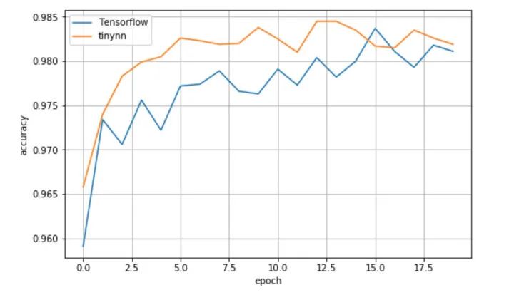
It can be seen that the effects of the two are not bad, and the accuracy of the test set converges to about 0.982, which is slightly better than Tensorflow in a single experiment.
summary
Tinynn related source code is in this repo( https://github.com/borgwang/tinynn )Inside. Currently supported:
-
Layer: full connection layer, 2D convolution layer, 2D deconvolution layer, MaxPooling layer, Dropout layer, BatchNormalization layer, RNN layer and activation functions such as ReLU, Sigmoid, Tanh, LeakyReLU and SoftPlus
-
loss: SigmoidCrossEntropy,SoftmaxCrossEntroy,MSE,MAE,Huber
-
optimizer: RAam, Adam, SGD, RMSProp, Momentum and other optimizers, and LRScheduler for dynamically adjusting learning rate is added
-
Common models such as mnist (classification), nn_paint (regression), DQN (reinforcement learning), AutoEncoder and DCGAN (unsupervised) are implemented. See tinynn/examples: https://github.com/borgwang/tinynn/tree/master/examples
tinynn still has a lot to improve. Due to the time limit, the author will maintain and update it in his spare time.
Of course, tinynn is just a "toy" version of the deep learning framework. A mature deep learning framework at least needs to support automatic derivation High computational efficiency (static language acceleration, supporting GPU acceleration), providing rich algorithm implementation, providing easy-to-use interfaces and detailed documents, etc. the starting point of this small project is more learning. In the process of designing and implementing tinynn, the author has learned a lot, including how to abstract, how to design component interfaces, how to implement more efficiently, and the specific details of algorithms Festival, etc. For the author, writing this small framework has another advantage in addition to understanding the design and implementation of the deep learning framework: in the follow-up, some new algorithms, new parameter initialization methods, new optimization algorithms and new network structure design can be quickly implemented on this small framework. If you are also interested in designing and implementing a deep learning framework, I hope this article will help you. You are also welcome to contribute code together with PR~
Appendix: Softmax cross entropy loss and gradient derivation
The cross entropy loss under multi classification is as follows:
Among them are the real value and the predicted value of the model, the number of samples and the number of categories. Since the real value is generally a one hot vector (0 except for the real category dimension of 1), the above formula can be simplified to
Where is the prediction probability representing the real category and the second sample category. That is, we need to calculate the sum of the logarithm of the prediction probability of each sample in the real category, and then take negative, which is the cross entropy loss. Next, we deduce how to solve the gradient of the loss with respect to the model output to represent the model output. In multi classification, Softmax is usually used to normalize the network output to a probability distribution, and the output after Softmax is
Substitute into the above loss function
Solving the gradient of output vector can be divided into target category dimension and non target category dimension. First, look at the dimension of the target category
Let's look at the dimensions of non target categories
You can see that for the target category dimension, the gradient is the output probability of the corresponding dimension model minus one, and for the non target category dimension, the gradient is the actual output probability of the corresponding dimension.
reference resources
-
Deep Learning, Goodfellow, et al. (2016)
-
Joel Grus - Livecoding Madness - Let's Build a Deep Learning Library
-
TensorFlow Documentation
-
PyTorch Documentation
If you feel useful, please like, collect and pay attention!