abstract
With the rapid development of global economy and stock market, stock investment has become one of the common financial management methods. In recent years, quantitative investment has attracted more and more attention because of its excellent discipline, accuracy, timeliness and systematicness. Compared with the western mature market, China's quantitative investment is still in its infancy, with some shortcomings and broad development prospects. At the same time, with the rapid development of artificial intelligence technology, there is a spark between machine learning and quantitative investment research. Therefore, aiming at the problem of quantitative stock selection, this paper combines machine learning and technical analysis, constructs a decision tree model, obtains the top ten stock portfolio, and makes an empirical test through the visual interface, The return of each stock in the portfolio and the total return of the portfolio are obtained respectively.
Keywords: decision tree; Quantitative stock selection; Visualization; sharpe ratio
1, Problem restatement
1.1 problem background
With the development of software technology and artificial intelligence technology, a large number of cumbersome data analysis and processing tasks have gradually changed from manual execution to computer automatic operation. This change is also quietly taking place in the financial sector in the pursuit of accuracy and efficiency. The subjective securities investment, once regarded as an art, has been gradually replaced by the quantitative investment strategy attached to the computer. Quantitative investment builds a mathematical model according to people's investment ideas and investment experience, and uses computers to process a large number of historical data to verify the effectiveness of the model in a short time. Only when the performance of the model meets the requirements in the historical data can it be further applied to the real transaction. Therefore, for stock investment, quantitative stock selection is the basis. Without good stock selection technology, the effect of quantitative investment will be greatly reduced.
1.2 problems to be solved
Design a quantitative stock selection system, which can arbitrarily select 28 first-class industries of Shenyin Wanguo, select the top 10 stocks based on the overall scale and investment efficiency method to build the portfolio, and conduct empirical test through the visual interface to obtain the return of each stock in the portfolio and the total return of the portfolio.
2, Problem analysis
The research object of the problem is any given multiple stocks, and the research content is quantitative stock selection strategy. The essence of this problem is to adopt the decision tree model in machine learning, use the preprocessed data over the years as the training set, select the appropriate label and gradually cut it into different subsets until all the training samples are classified correctly, classify and predict the data of the next year, and then construct the portfolio according to the classification results. The core of the model is to select appropriate features, that is, feature extraction.
3, Symbol description and noun definition
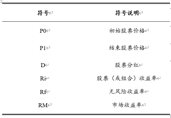
4, Model establishment and solution
4.1 data preprocessing
Data preprocessing includes data cleaning and data visualization and analysis.
There are two annexes in total. The data in the annex gives the relevant information of Shenyin Wanguo's 28 primary industry stocks:
Annex 1: stock code of Shenwan industry;
Annex 2: stock market data of shenwanyi industry (from January 1, 2021 to June 30, 2021);
There are invalid values in Annex 1, so Annex 1 needs to clean and sort out the data, and use Excel and Python software to preprocess the data as follows. Using the above data, the problem is solved and analyzed.
4.1. 1 data cleaning
Some stocks in Annex 1 are delisted, but their codes are still. The specific codes are as follows: 688509
688688, 688385, 688670, 688148, 688071, 688778 and 688779 must be deleted.
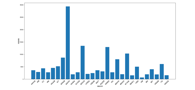
4.1. 2 data visualization and analysis
Annex 1 the number of constituent shares of each primary industry of Shenyin Wanguo is shown in Figure 1.

Figures 2, 3 and 4 show the rise and fall, income index and trading volume of Shenyin Wanguo's primary industries.


4.2 characteristic Engineering
There are generally many indicators to measure a stock. Here we select five indicators: yield, alpha, sharp ratio, maximum pullback and beta.
The yield is the ratio between the stock return (stock appreciation + dividend) and the initial investment. The higher the value, the better the stock performance without considering the risk.
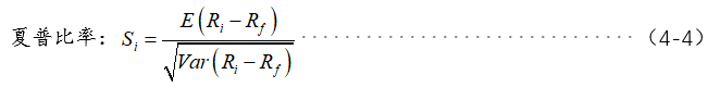
Sharp ratio describes the degree of return that a stock or portfolio can obtain under unit risk compared with risk-free return. It normalizes the risk of stocks or portfolios to better compare the effectiveness of portfolios. The higher the value, the better the performance of the stock or portfolio considering the risk.
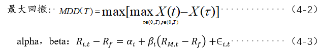
Pullback describes the maximum loss that investors may face and is an important risk indicator to measure the anti risk ability of the portfolio. The maximum drawdown (MDD) is defined as the maximum value of the rate of return pullback at any historical point in the selected cycle. The lower the pullback value, the better.
Alpha measures the active return (excess return) of a stock or portfolio relative to the market. alpha=0 indicates that the performance is consistent with the market. Alpha < 0 indicates that the return is worse than the market. Alpha > 0 indicates that stocks or portfolios outperform the market. alpha=1%, equivalent to 1% higher than the market income in the same period.
Beta measures the correlation between the stock or portfolio and the market trend, and explains the return of the stock or portfolio from the market (market return). The beta of the market is 1. Beta > 1 means that the stock or market is more related to the market trend, and the shock is more intense. Beta < 1 means that it is either less relevant to the market trend, or the shock is smaller than the market.
4.3 model establishment and solution
4.3. 1. Establishment of model
Here, the machine learning strategy is adopted and the support vector machine model is used. The specific algorithm is described as follows:
Table 1 specific algorithm description of Niubi
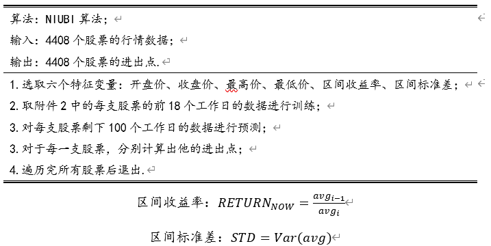
The results obtained by the above algorithm support the next calculation
The number of stocks in Annex 2 is 4408. Firstly, calculate the rate of return for each stock. The specific algorithm description is shown in Table 2:
Table 2 description of return algorithm

Similarly, according to the above algorithm process, the maximum stock pullback rate, alpha and beta values can be calculated:
4.3. 2 solution of model
Calculate the stocks in Annex II respectively, and the final results are as follows (only the top 15 are ranked, and the calculation results retain one digit after the decimal point):
Table 3 ranking of stock returns
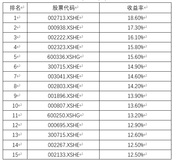
Table 4 ranking of maximum stock pullback rate

Table 5 ranking of maximum stock pullback rate

The final total score is calculated by the following formula:
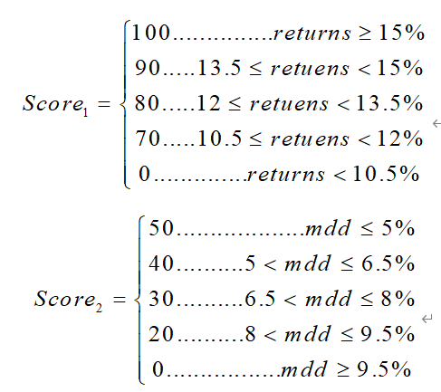
The scoring results are as follows:

According to the following formula, the sharp ratio of the portfolio is 1.43, indicating that the portfolio is a better portfolio after comprehensive income and risk.
4.3. 3 performance evaluation of the model
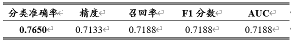
The classification accuracy, precision, recall, F1 score and AUC value were used as the indexes to evaluate the support vector machine. The accuracy rate is the proportion of the samples with correct classification to the total number, the accuracy is the proportion of the number of samples with correct prediction to the number of samples with positive prediction, the recall rate is the proportion of the number of samples with correct prediction to the actual number of samples with positive prediction, the F1 score is the harmonic average of the accuracy and recall rate, and the AUC is the area under the ROC curve, the larger the better. The model performance is shown in Table 6.
Table 6 model evaluation
5, Evaluation and improvement of model
5.1 model evaluation
5.1. 1 advantages of the model
(1) Fast speed: the amount of calculation is relatively small, and it is easy to transform into classification rules As long as you walk down the tree root to the leaf, the splitting conditions along the way can uniquely determine a predicate of classification;
(2) High accuracy: the mined classification rules are accurate and easy to understand. The decision tree can clearly display which fields are important, that is, understandable rules can be generated;
(3) Can handle continuous and category fields;
(4) No domain knowledge and parameter assumptions are required;
(5) Suitable for high-dimensional data.
5.1. 2 disadvantages of the model
(1) For the data with different sample numbers in each category, the information gain tends to the characteristics with more values;
(2) Easy over fitting;
(3) Ignore dependencies between attributes.
5.2 model improvement
Overfitting is an important practical difficulty for decision tree learning and many other learning algorithms. There are several ways to avoid over fitting in decision tree learning. They can be divided into two categories:
(1) Stop the growth tree method as soon as possible and stop the growth tree before ID3 algorithm perfectly classifies the training data;
(2) Post pruning method allows the tree to over fit the data, and then post prune the tree.
Although the first method may seem more direct, the second method of post pruning over fitted trees has proved more successful in practice. This is because in the first method, it is difficult to accurately estimate when to stop growing the tree. Whether we get the correct size of the tree by stopping early or pruning later, a key problem is what criteria to use to determine the final correct size of the tree. Solutions to this problem include:
(1) A set of separate samples, which are different from the training samples, are used to evaluate the utility of pruning nodes from the tree by post pruning method;
(2) Use all available data for training, but conduct statistical tests to estimate whether expanding (or pruning) a specific node may improve the performance on instances outside the training set;
(3) A clear standard is used to measure the complexity of training samples and decision tree coding. When the length of this coding is the smallest, stop growing the tree.
6, Application of model
The financial industry can use the decision tree for loan risk assessment, the insurance industry can use the decision tree for insurance promotion prediction, the medical industry can use the decision tree to generate auxiliary diagnosis and disposal models, and so on.
reference
[1] Li Bin, Shao Xinyue, Li eryang Research on fundamental quantitative investment driven by machine learning [J] China industrial economy, 2019 (08): 61-79
[2] Huang Hongyuan, Wang Mei Multi factor stock selection model based on multiple regression analysis [J] Journal of assimilation demonstration college, 2016
[3] Ding Peng Quantitative investment strategy and technology [M]. Beijing: Electronic Industry Press, 2014,24-29
[4] Zhou Zhihua Machine learning [M] · Beijing: Tsinghua University Press, 2016121-137
[5] Wang yuanfan, Shi Yong, Xue Zhi Research on port scanning malicious traffic detection based on decision tree [J] Communication technology, 2020,53 (08): 2002-2005
[6] Li Kai, Tan Haibo, Wang Haiyuan, Xie Yuman, Huang Hongqiao, bu Wenbin, Tan Cong, Peng Xiao, Guo Guang, Liu mouhai, Chen Hao A main network line state detection method, system and medium based on decision tree [P] Hunan Province: cn111612149a, September 1, 2020
[7] Zhou Jian Empirical Study on multi factor stock selection model based on SVM algorithm [D] Zhejiang Business University, 2017
[8] Cao Zhengfeng, Ji Hong, Xie bangchang Using random forest algorithm to realize the selection of high-quality stocks [J] The capital economy
Appendix 1
1. Data cleaning
1.	import pandas as pd
2.	from jqdatasdk import *
3.	from jqdatasdk.api import get_price, get_query_count
4.	from numpy import nan
5.
6.	auth('13259391862', '2001720Lmt')
7.	get_query_count()
8.
9.	industry_code = pd.read_csv("Industries.csv", index_col=0)
10.	stock_code = pd.read_csv("total.csv",index_col=0,dtype=str)
11.	stock_code.columns = [x for x in industry_code.index]
12.
13.	for j in stock_code.index:
14.	    for i in stock_code.columns:
15.	        try:
16.	            if stock_code[i][j] is not nan:
17.	                prices = get_price(
18.	                    stock_code[i][j],
19.	                    start_date='2021-01-01',
20.	                    end_date='2021-06-30',
21.	                    frequency='1d',
22.	                    fields=['open', 'close', 'low', 'high', 'avg'])
23.	                prices.to_csv(stock_code[i][j] + '.csv')
24.	                print("Data entry" + stock_code[i][j] + "Completed...")
25.	            else:
26.	                continue
27.	        except:
28.	            print(stock_code[i][j] + "Unable to enter...")
2. Tactics
1.	from datetime import timedelta
2.	import jqdata
3.	import scipy.optimize as optimize
4.	import statsmodels.api as sm
5.	from jqdatasdk import valuation, balance, income, indicator, get_fundamentals
6.
7.
8.	# Initialize functions, set benchmarks, etc
9.	def initialize(context):
10.	    set_benchmark('000300.XSHG')
11.	    # Enable dynamic reversion mode (real price)
12.	    set_option('use_real_price', True)
13.	    # Output content to log info()
14.	    log.info('The initial function starts running and the global is run only once')
15.	    # The handling fee for each transaction of stocks is: 0.03% of the commission when buying, 0.03% of the commission when selling and 1 / 1000 of the stamp duty. The minimum commission for each transaction is 5 yuan
16.	    set_order_cost(OrderCost(close_tax=0.001, open_commission=0.0003, close_commission=0.0003, min_commission=5),
17.	                   type='stock')
18.	    # Operation before opening
19.	    run_daily(before_market_open,time='before_open',
20.	reference_security='000300.XSHG')
21.	    # Run after closing
22.	run_daily(after_market_close,time='after_close',
23.	reference_security='000300.XSHG')
24.	    set_parameters()
25.
26.
27.	## Run function before opening
28.	def before_market_open(context):
29.	    # Output run time
30.	log.info('Function run time(before_market_open): ' +
31.	str(context.current_dt.time()))
32.
33.	factors = ['CMC', 'MC', 'CMC/C', 'TOE/MC',
34.	'PB', 'NP/MC', 'TP/MC', 'TA/MC',
35.	'OP/MC', 'CRF/MC', 'PS', 'OR/MC',
36.	               'RP/MC', 'TL/TA', 'TCA/TCL', 'PE',
37.	'OR*ROA/NP', 'GPM', 'IRYOY', 'IRA',
38.	'INPYOY', 'INPA', 'NPM', 'OPTTR',
39.	               'C', 'CC', 'PR', 'PRL', 'ROE',
40.	'ROA', 'EPS', 'ROIC', 'ZYZY']
41.	    # Factor get factor parameters
42.	    theta, mu, sigma = getThetaByFeatures(context, factors)
43.	    # Factor stock selection
44.	    if sum(theta) == 0:
45.	        return
46.	    stock_list = selectStocks(context, factors, theta, mu, sigma)
47.	    stock_list = unStartWith300(stock_list)
48.	    stock_list = filter_paused_and_st_stock(stock_list)
49.	    stock_list = filter_limitup_stock(context, stock_list)
50.	    stock_list = filter_limitup_stock(context, stock_list)
51.	    g.stock_to_buy = stock_list
52.
53.
54.	## Run function after closing
55.	def after_market_close(context):
56.	log.info(str('Function run time(after_market_close):' +
57.	str(context.current_dt.time())))
58.	    # Get all transaction records of the day
59.	    trades = get_trades()
60.	    for _trade in trades.values():
61.	        log.info('Transaction record:' + str(_trade))
62.	    log.info('End of day')
63.	    log.info('#######################################################')
64.
65.
66.	# Set parameters
67.	def set_parameters():
68.	    g.period = 10
69.	    g.buyStockCount = 50
70.	    g.stock_to_buy = []
71.	    g.days = 0
72.
73.
74.	# transaction
75.	def trades(context, data, stock_list):
76.	    # Sell stocks that are not on the list
77.	    for stock in context.portfolio.positions.keys():
78.	        if stock not in stock_list:
79.	            order_target_value(stock, 0)
80.
81.	    # Calculate the quantity that still needs to be purchased
82.	    num_to_buy = len(stock_list) - len(context.portfolio.positions.keys())
83.	    if num_to_buy == 0:
84.	        return
85.	    # Cash distribution
86.	    cash = context.portfolio.available_cash
87.	    cash = 1.0 * cash / num_to_buy
88.	    for stock in stock_list:
89.	        if stock not in context.portfolio.positions.keys():
90.	            order_target_value(stock, cash)
91.
92.
93.	# Daily operation
94.	def dailyRunning(context, data):
95.	    # Filter price limit stocks
96.	    stock_list = g.stock_to_buy
97.	    stock_list = filter_limitup_stock(context, stock_list)
98.	    stock_list = filter_limitup_stock(context, stock_list)
99.	    stock_list = stock_list[:g.buyStockCount]
100.	    # transaction
101.	    if g.days % g.period == 0:
102.	        trades(context, data, stock_list)
103.	    g.days += 1
104.	    pass
105.
106.
107.	## Run function at opening
108.	def handle_data(context, data):
109.	    # Get current time
110.	    hour = context.current_dt.hour
111.	    minute = context.current_dt.minute
112.
113.	    # Every day at 14:50 p.m
114.	    if hour == 14 and minute == 50:
115.	        # Daily operation
116.	        dailyRunning(context, data)
117.
118.
119.	# Remove gem
120.	def unStartWith300(stockspool):
121.	    return [stock for stock in stockspool if stock[0:3] != '300']
122.
123.
124.	# Filter suspended, ST stocks and other stocks with delisting labels
125.	def filter_paused_and_st_stock(stock_list):
126.	    current_data = get_current_data()
127.	    return [stock for stock in stock_list if not current_data[stock].paused and not current_data[stock].is_st
128.	            and 'ST' not in current_data[stock].name and '*' not in current_data[stock].name and 'retreat' not in
129.	            current_data[stock].name]
130.
131.
132.	# Filter trading stocks
133.	def filter_limitup_stock(context, stock_list):
134.	    last_prices = history(1, unit='1m', field='close', security_list=stock_list)
135.	    current_data = get_current_data()
136.
137.	    # The stock already in the position is not filtered even if it rises or falls, so as to avoid that the stock can be bought again, but it will be filtered and lead to the selection of other stocks
138.	    return [stock for stock in stock_list if stock in context.portfolio.positions.keys()
139.	            or last_prices[stock][-1] < current_data[stock].high_limit]
140.
141.
142.	# Filter down limit stocks
143.	def filter_limitdown_stock(context, stock_list):
144.	last_prices = history(1, unit='1m', field='close',
145.	security_list=stock_list)
146.	    current_data = get_current_data()
147.	    return [stock for stock in stock_list if stock in context.portfolio.positions.keys()
148.	            or last_prices[stock][-1] > current_data[stock].low_limit]
149.
150.
151.	# Cost function
152.	def costFunction(theta, X, y):
153.	    m = len(y)
154.	    tmp_theta = theta.reshape(len(theta), 1).copy()
155.	    temp = X.dot(tmp_theta)
156.	    J = sum(np.square(temp - y)) / 2.0 / m
157.	    return J
158.
159.
160.	# gradient
161.	def gradient(theta, X, y):
162.	    # Number of samples
163.	    m = y.size
164.	    # Copy of parameters
165.	    tmp_theta = theta.reshape(len(theta), 1).copy()
166.	    # Prediction function
167.	    h = dot(X, tmp_theta)
168.	    # Gradient calculation
169.	    grad = 1.0 / m * X.T.dot(h - y)
170.	    grad = grad.flatten()
171.	    return grad
172.
173.
174.	# Cost function (regularization)
175.	def costFunctionReg(theta, X, y, mylambda):
176.	    m = len(y)
177.	    tmp_theta = theta.reshape(len(theta), 1).copy()
178.	    temp = X.dot(tmp_theta)
179.	    J = sum(np.square(temp - y)) / 2.0 / m + 1.0 * mylambda / 2 / m * sum(tmp_theta ** 2)
180.	    return J
181.
182.
183.	# gradient
184.	def gradientReg(theta, X, y, mylambda):
185.	    # Number of samples
186.	    m = y.size
187.	    # Copy of parameters
188.	    tmp_theta = theta.reshape(len(theta), 1).copy()
189.	    # Prediction function
190.	    h = dot(X, tmp_theta)
191.	    # Gradient calculation
192.	    grad = 1.0 / m * X.T.dot(h - y) + 1.0 * mylambda / m * tmp_theta
193.	    grad = grad.flatten()
194.	    return grad
195.
196.
197.	# Mean normalization
198.	def featureNormalize(X):
199.	    mu = mean(X)
200.	    sigma = std(X)
201.	    X_norm = 1.0 * (X - mu) / sigma
202.	    return X_norm, mu, sigma
203.
204.
205.	# The fitting parameters are obtained
206.	def getThetaByFeatures(context, factors):
207.	    period = g.period
208.	    period = 1
209.	    # Last warehouse adjustment date
210.	    yesterday = context.previous_date
211.	    daysBefore = yesterday - timedelta(days=period * 2)  # period * 2
212.	    trade_days = jqdata.get_trade_days(start_date=daysBefore, end_date=yesterday)
213.	    log.info(trade_days)
214.	    log.info(trade_days[-period - 1:])
215.	    # cycle
216.	    trade_days = trade_days[-period - 1:]
217.	    # Start and end date
218.	    start_date = trade_days[0]
219.	    end_date = trade_days[-1]
220.	    # Get the factor data of the stock on the last position adjustment day and construct the feature combination
221.	    x_df = get_factors(start_date, factors)
222.	    # Feature scaling
223.	    # Get the increase of stocks on the last position adjustment day and build the result portfolio
224.	    stock_list = x_df.index.tolist()
225.	    df = get_price(stock_list, start_date=start_date, end_date=end_date, frequency='daily', fields=['close'])['close']
226.	    y_se = df.ix[-1] / df.ix[0] - 1
227.	    y = y_se[~ np.isnan(y_se)]
228.	    x = x_df.ix[y.index.tolist()]
229.	    n = len(x_df.columns)
230.	    m = len(y)
231.	    X_norm, mu, sigma = featureNormalize(x)
232.	    X = sm.add_constant(X_norm)
233.	    for i in X.columns:
234.	        X[i] = np.nan_to_num(X[i])
235.	    X = np.c_[X]
236.	    y = np.c_[y]
237.	    # Initialization parameters
238.	    initial_theta = np.zeros(n + 1)
239.	    # Regularization parameters
240.	    mylambda = 1
241.	    opts = {'disp': False,
242.	            'xtol': 1e-05,
243.	            'eps': 1.4901161193847656e-08,
244.	            'return_all': False,
245.	            'maxiter': None}
246.	    result = optimize.minimize(costFunctionReg, initial_theta, args=(X, y, mylambda), method='Newton-CG',
247.	                               jac=gradientReg, hess=None, hessp=None, tol=None, callback=None, options=opts)
248.	    theta = result.x
249.	    return theta, mu, sigma
250.
251.
252.	# Get factor data
253.	def get_factors(fdate, factors):
254.	    # stock_set = get_index_stocks('000300.XSHG',fdate)
255.	    q = query(
256.	        valuation.code,  # Stock code
257.	        valuation.circulating_market_cap,  # CMC current market value
258.	        valuation.market_cap,  # MC total market value
259.	        valuation.circulating_market_cap / valuation.capitalization * 10000,  # CMC/C current market value (100 million) / total share capital (10000) (closing price)
260.	        balance.total_owner_equities / valuation.market_cap / 100000000,  # TOE/MC owner's equity per yuan
261.	        valuation.pb_ratio,  # PB price to book ratio
262.	        income.net_profit / valuation.market_cap / 100000000,  # NP/MC owner's net profit per yuan
263.	        income.total_profit / valuation.market_cap / 100000000,  # TP/MC total profit per yuan
264.	        balance.total_assets / valuation.market_cap / 100000000,  # TA/MC total assets per yuan
265.	        income.operating_profit / valuation.market_cap / 100000000,  # OP/MC operating profit per yuan
266.	        balance.capital_reserve_fund / valuation.market_cap / 100000000,  # CRF/MC capital reserve per yuan
267.	        valuation.ps_ratio,  # PS market sales rate
268.	        income.operating_revenue / valuation.market_cap / 100000000,  # OR/MC operating income per yuan
269.	        balance.retained_profit / valuation.market_cap / 100000000,  # RP/MC undistributed profit per yuan
270.	        balance.total_liability / balance.total_sheet_owner_equities,  # TL/TA asset liability ratio
271.	        balance.total_current_assets / balance.total_current_liability,  # TCA/TCL current ratio
272.	        valuation.pe_ratio,  # PE P / E ratio
273.	        income.operating_revenue * indicator.roa / income.net_profit,  # OR*ROA/NP total asset turnover
274.	        indicator.gross_profit_margin,  # GPM gross margin on sales
275.	        indicator.inc_revenue_year_on_year,  # Yoy growth rate of IRYOY operating revenue (%)
276.	        indicator.inc_revenue_annual,  # Month on month growth rate of IRA operating revenue (%)
277.	        indicator.inc_net_profit_year_on_year,  # Year on year growth rate of INPYOY net profit (%)
278.	        indicator.inc_net_profit_annual,  # Month on month growth rate of INPA net profit (%)
279.	        indicator.net_profit_margin,  # NPM net profit margin (%)
280.	        indicator.operation_profit_to_total_revenue,  # OPTTR operating profit / total operating revenue (%)
281.	        valuation.capitalization,  # C total share capital
282.	        valuation.circulating_cap,  # CC circulating share capital (10000 shares)
283.	        valuation.pcf_ratio,  # PR market rate
284.	        valuation.pe_ratio_lyr,  # PRL P / E ratio LYR
285.	        indicator.roe,  # ROE return on net assets (%)
286.	        indicator.roa,  # ROA net interest rate of total assets (%)
287.	        indicator.eps,  # EPS earnings per share
288.	        # ROIC
289.	        # EBIT = net profit + Interest + tax
290.	        # ROIC
291.	        (income.net_profit + income.financial_expense + income.income_tax_expense) / (
292.	                balance.total_owner_equities + balance.shortterm_loan + balance.non_current_liability_in_one_year + balance.longterm_loan + balance.bonds_payable + balance.longterm_account_payable),
293.	        (
294.	                balance.accounts_payable + balance.advance_peceipts + balance.other_payable - balance.account_receivable - balance.advance_payment - balance.other_receivable) / (
295.	                balance.total_owner_equities + balance.shortterm_loan + balance.non_current_liability_in_one_year + balance.longterm_loan + balance.bonds_payable + balance.longterm_account_payable)
296.	    ).filter(
297.	        # valuation.code.in_(stock_set),
298.	        valuation.circulating_market_cap
299.	    )
300.	    fdf = get_fundamentals(q, date=fdate)
301.	    fdf.index = fdf['code']
302.	    fdf.columns = ['code'] + factors
303.	    # Row: select all, column, and return all factors except stock code
304.	    return fdf.iloc[:, 1:]
305.
306.	# Stock selection method
307.	def selectStocks(context, factors, theta, mu, sigma):
308.	    x_df = get_factors(context.current_dt, factors)
309.	    X_norm = (x_df - mu) / sigma
310.	    X = sm.add_constant(X_norm)
311.	    for i in X.columns:
312.	        X[i] = np.nan_to_num(X[i])
313.	    # Copy of parameters
314.	    tmp_theta = theta.reshape(len(theta), 1).copy()
315.	    # Prediction function
316.	    h = dot(X, tmp_theta)
317.	    # Result assignment, predicted increase
318.	    X['predict'] = h
319.	X = X.sort(columns=['predict'], ascending=[False])
320.	return X.index.tolist()
Appendix 2
List of attachments:
Appendix 1: Appendix 1: stock code of shenwanyi industry csv
Appendix 2: Appendix 2: stock market data of shenwanyi industry (from January 1, 2021 to June 30, 2021)
Annex 3: Pictures
See upload resources for the appendix
Welcome to join me for wechat learning and discussion