Chapter 4 advanced linear regression algorithm

   the solution of multivariable linear regression algorithm is far away from univariate linear regression algorithm, and overcomes the limitation of univariate linear regression algorithm with only one characteristic variable in practical application, so it is widely used.
   there are specific requirements for variables in the conventional solution of multivariable linear regression, but it is impossible to meet this requirement in practical application. At the same time, there are problems such as over fitting. Therefore, on the basis of basic solution, regularization, ridge regression and Lasso regression need to be introduced to further optimize and expand the solution of multivariable linear regression algorithm.

4.1 multivariable linear regression algorithm

4.1.1 least square solution of multivariable linear regression algorithm

Basic model:
  hθ(x)=θ0+θ1x1+θ2x2+θ3x3+...+θnxn

• h θ (x) Table Shiyi θ Is a parameter, θ 0 θ 1， θ 2， θ 3，… θ n is the regression parameter to be solved
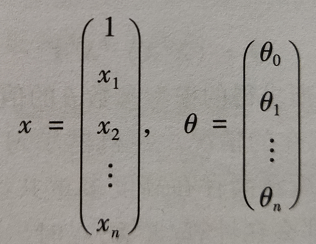
     since there are n characteristic variables x, x can be expressed in the form of matrix:
  
  Of which:
  
  Cost function:
  
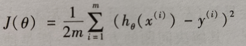
• m: Number of training samples in the training set
• (x(i),y(i)): the ith training sample. Superscript i is the index, indicating the ith training sample

solve θ:

Get:

• Here, it is assumed that the rank of matrix X is generally n+1, that is, (XTX) - 1 exists
• (XTX) - 1 causes of irreversibility:
     there is a high degree of multicollinearity between independent variables, such as x2=2x1
    there are too many characteristic variables, too high complexity and relatively few training data. Solution: use regularization and ridge regression

4.1.2 Python implementation of multivariable linear regression: fitting of cinema audience (I)

Visualization of multivariate data

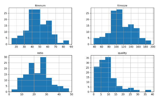
1. Histogram (including imported data)

# histogram
"""
    xlabelsize=12: X Shaft size
    ylabelsize=12: Y Shaft size
    figsize=(12,7): Size of the entire drawing
"""
df = pd.read_csv('D:/PythonProject/machine/data/3_film.csv')
df.hist(xlabelsize=12,ylabelsize=12,figsize=(12,7))
plt.show()

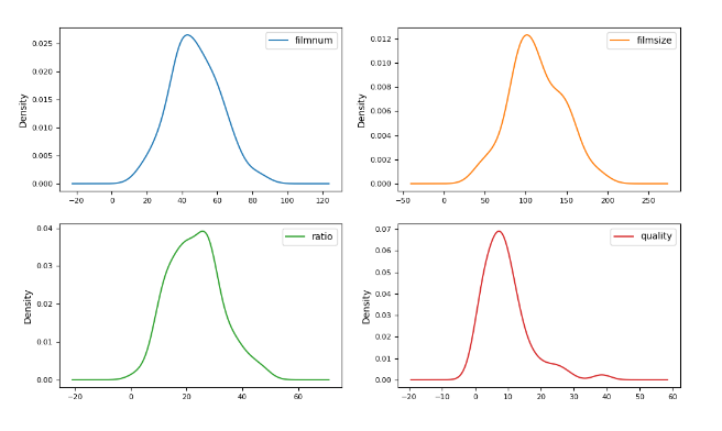
1. Density map

# Density map
"""
    kind: Graphic type
    subplots=True: Multiple subgraphs need to be drawn
    layout=(2,2): Number of subgraphs drawn 2*2
    sharex=False: Subgraphs are not shared X axis
    fontsize=8: font size
"""
df.plot(kind="density",subplots=True,layout=(2,2),sharex=False,fontsize=8,figsize=(12,7))
plt.show()

1. Box diagram

# Box diagram
df.plot(kind='box',subplots=True,layout=(2,2),sharex=False,sharey=False,fontsize=8,figsize=(12,7))
plt.show()

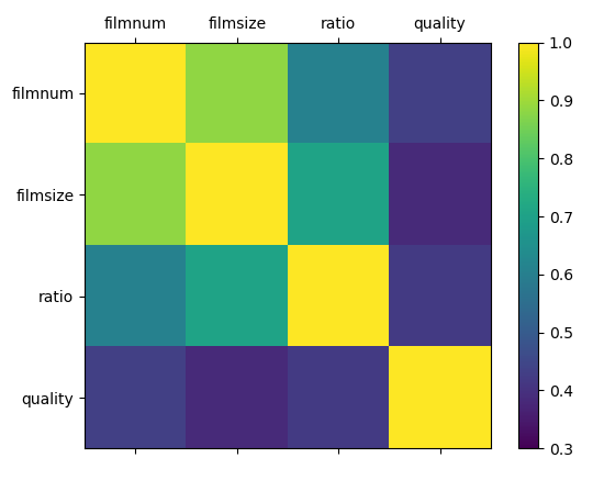
1. Correlation coefficient thermodynamic diagram

# Correlation coefficient thermodynamic diagram
# Set variable name
names = ['filmnum','filmsize','ratio','quality']
# Calculate the correlation coefficient matrix between variables
correlations = df.corr()
# Call figure to create a drawing object
fig = plt.figure()
# Call the Sketchpad to draw the first sub graph
ax = fig.add_subplot(111)
# Draw thermal diagram from 0.3 to 1
cax = ax.matshow(correlations,vmin=0.3,vmax=1)
# Set the heat map generated by matshow as a color gradient bar
fig.colorbar(cax)
# Generate 0-4 in steps of 1
ticks = np.arange(0,4,1)
# Generate x/y axis scale
ax.set_xticks(ticks)
ax.set_yticks(ticks)
# Generate x/y axis labels
ax.set_xticklabels(names)
ax.set_yticklabels(names)
plt.show()

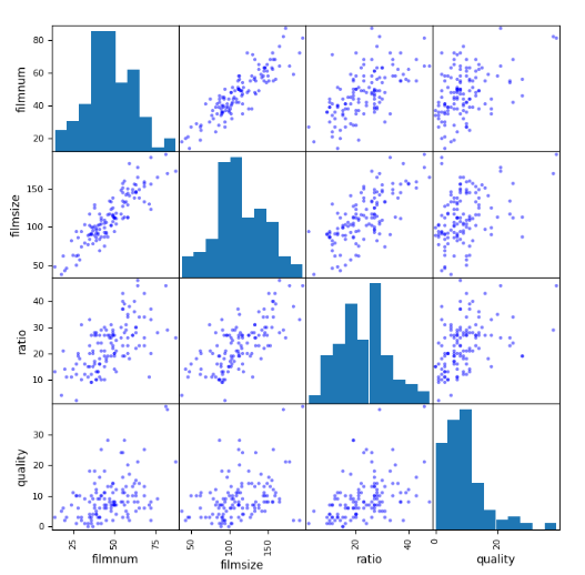
1. Scatter matrix

# Scatter matrix
# Plot scatter matrix
"""
    df: data sources 
    figsize=(8,8): Graphic size
    c='b': Color of scatter points
"""
scatter_matrix(df,figsize=(8,8),c='b')
plt.show()

Data fitting and prediction of multivariable linear regression algorithm

1. Select characteristic variables and response variables, and divide the data

df = pd.read_csv('D:/PythonProject/machine/data/3_film.csv')
# Select the X variable in data
"""
    :,1:4: Represents the selected dataset 2-4 column
"""
X = df.iloc[:,1:4]
# Set target to y
y = df.filmnum
# Convert X and y into array form for easy calculation
X = np.array(X.values)
y = np.array(y.values)
# The test samples are constructed with 25% of the data, and the rest are used as training samples
X_train,X_test,y_train,y_test = train_test_split(X,y,test_size=0.25,random_state=1)
print(X_train.shape,X_test.shape,y_train.shape,y_test.shape)

(94, 3) (32, 3) (94,) (32,)

1. Perform linear regression operation and output the results

lr = LinearRegression()
lr.fit(X_train,y_train)
print('a={}\nb={}'.format(lr.coef_,lr.intercept_))

a=[ 0.37048549 -0.03831678 0.23046921]
b=4.353106493779016

1. According to the calculated parameters, the test set is predicted

y_hat = lr.predict(X_test)
print(y_hat)

[20.20848598 74.31231952 66.97828797 50.61650336 50.53930128 44.72762082
57.00320531 35.55222669 58.49953514 19.43063402 27.90136964 40.25616051
40.81879843 40.01387623 24.56900454 51.36815239 38.97648053 39.25651308
65.4877603 60.82558336 54.29943364 40.45641818 29.69241868 49.29096985
44.60028689 48.05074366 35.23588166 72.29071323 53.79760562 51.94308584
46.42621262 73.37680499]

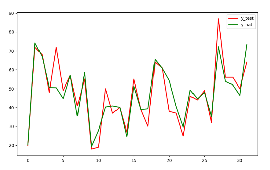
1. Comparison of actual values of corresponding variables in test set and prediction set

# Create t variable
t = np.arange(len(X_test))
# Draw y_test curve
plt.plot(t,y_test,'r',linewidth=2,label='y_test')
# Draw y_hat curve
plt.plot(t,y_hat,'g',linewidth=2,label='y_hat')
plt.legend()
plt.show()

1. Evaluate the prediction results

# Output method I of goodness of fit R2
print('R2_1={}'.format(lr.score(X_test,y_test)))
# Output method 2 of goodness of fit R2
print('R2_2={}'.format(r2_score(y_test,y_hat)))
# Calculate MAE
print('MAE={}'.format(metrics.mean_absolute_error(y_test,y_hat)))
# Calculate MSE
print('MSE={}'.format(metrics.mean_squared_error(y_test,y_hat)))
# Calculate RMSE
print('RMSE={}'.format(np.sqrt(metrics.mean_squared_error(y_test,y_hat))))

R2_1=0.8279404383777595
R2_2=0.8279404383777595
MAE=4.63125112009528
MSE=46.63822281456598
RMSE=6.8292183165107545

Data file:
Link: https://pan.baidu.com/s/1TVPNcRKgrDttDOFV8Q2iDA
Extraction code: h4ex