I. limit learning machine

Single hidden layer feedback neural network has two outstanding capabilities:

(1) The complex mapping function f: x ^ t can be fitted directly from the training samples

(2) it can provide models for a large number of natural or artificial phenomena that are difficult to deal with by traditional classification parameter technology. However, the single hidden layer feedback neural network lacks a relatively fast learning method. Each iteration of the error back propagation algorithm needs to update n x(L+ 1) +L x (m+ 1), which takes much less time than the tolerated time. It is often seen that it takes hours, days or more to train a single hidden layer feedback neural network.
Based on the above reasons, Professor Huang guangbin has conducted in-depth research on single hidden layer feedback neural network
Two bold theories have been developed and proved:

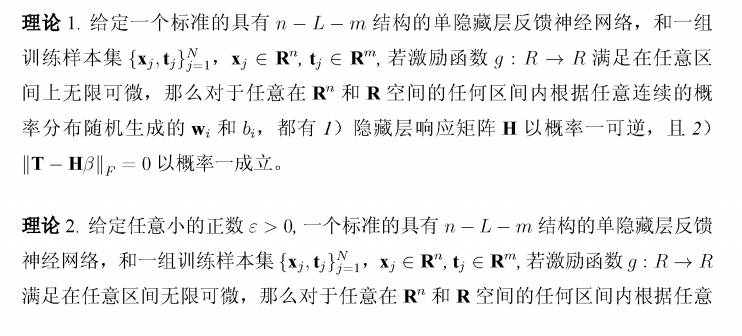
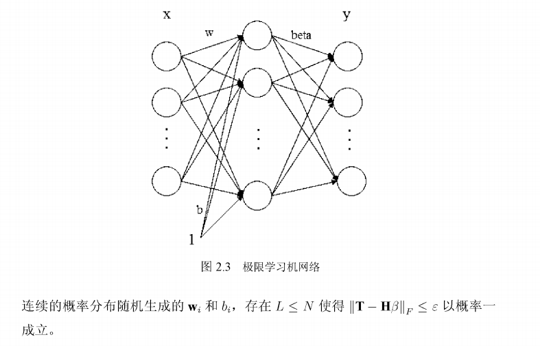
From the above two theories, we can see that as long as the excitation function g:R ^ R is infinitely differentiable in any interval, wt and bt can be randomly generated according to any continuous probability distribution from the n-dimension of R and any interval of R space, that is, the single hidden layer feedforward neural network does not need to adjust wt and bt; And because of the formula | th * beta||_ If f = 0, we find that the offset of the output layer is no longer required. Then a new but hidden layer feedback neural network is shown in Figure 2.3.
Compared with FIG. 2.2, the output layer bias bs is missing, and the input weight w and hidden layer bias bi are generated randomly without adjustment, so only the output weight beta of the whole network is not determined. So extreme learning machine
emerge as the times require. Make the output of the neural network equal to the sample label, as shown in equation (2-11)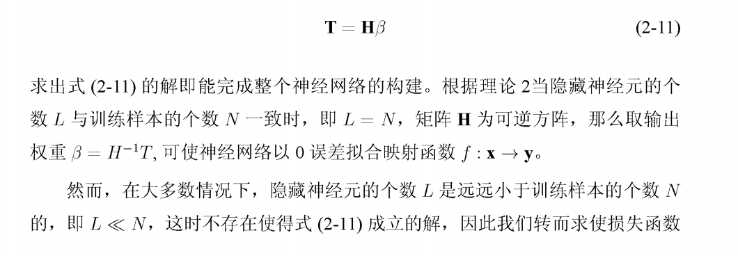

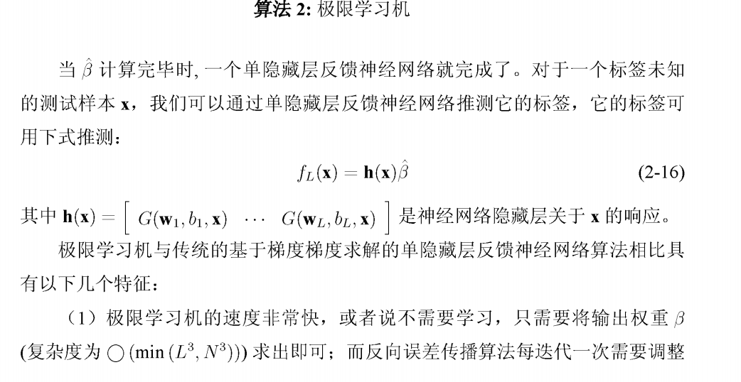
n x(L+1) +Lx(m+1), and in order to ensure the stability of the system, the back-propagation algorithm usually selects a small learning rate, which greatly prolongs the learning time. Therefore, the extreme learning machine has great advantages in this method. In the experiment, the extreme learning machine often completes the operation in a few seconds. Some classical algorithms spend a lot of time in training a single hidden layer neural network, even a small application. It seems that these algorithms have an insurmountable virtual speed barrier.

(2) In most applications, the generalization ability of limit learning machine is greater than that of gradient based algorithms such as error back propagation algorithm.
(3) the traditional gradient based algorithm needs to face problems such as local minimization, appropriate learning rate, over fitting and so on. The limit learning machine directly constructs a single hidden layer feedback neural network in one step to avoid these difficult problems.
Because of these advantages, the majority of researchers are very interested in extreme learning machine, which makes the theory of extreme learning machine develop rapidly and its application is constantly expanding in recent years.

2, Bottle sea squirt algorithm

Bottlenose sea squirt is a transparent barrel like creature, which is similar to jellyfish. It moves by absorbing water and spraying water. Because it lives in the deep sea of the cold zone, it has caused some trouble to our research. However, this does not affect our research on it. In the deep sea, the bottle sea squirt exists in the form of bottle sea squirt chain, which is one of the group behaviors we are interested in.

Firstly, we divide the bottle sea squirt chain into two groups: 1. Leaders; 2. Followers.

The leader is the front part of the bottle sea squirt chain; The follower is the back end of the bottle sea squirt chain.

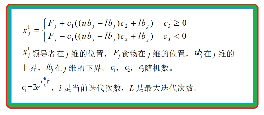
First, the leader's position is the same as the new formula:

　　

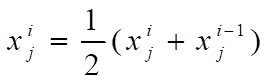
Update follower location

　　

3, Code

% Transpose to adapt to the network structure
%%  data normalization 
p_train=p_train';%n*m data n Is the number of input features, m Is the number of samples
t_train=t_train';%n*m data n Is the number of input features, m Is the number of samples
% [p_train, ps_input] = mapminmax(p_train,0,1);
% [t_train, ps_output] = mapminmax(t_train,0,1);
p_test=p_test';
% [p_test ] = mapminmax(p_test' ,0,1);
% p_test = mapminmax('apply',p_test',ps_input);

%% Network establishment and training
% Using the loop, set the number of neurons in different hidden layers
nn=[7 11 14 18];
shuchu=1;%Output result dimension
for i=1:4
    threshold=[0 2;0 2];%How many? n How many?[0,1]
    % establish Elman The hidden layer of neural network is nn(i)Neurons
    net=newelm(threshold,[nn(i),shuchu],{'tansig','purelin'});%Several outputs
    % Set network training parameters
    net.trainparam.epochs=2000;
    net.trainparam.show=20;
    net.trainParam.showWindow = false;
net.trainParam.showCommandLine = false; 
    % Initialize network
    net=init(net);
    % Elman Network training
    net=train(net,p_train,t_train);
    % Forecast data
    y=sim(net,p_test)*1000/25;%% Data inverse normalization
%     y= mapminmax('reverse',y,ps_output);
    % calculation error
%     error(i,:)=y'-t_test;
        rmse(i)=sqrt(mse(y'-t_test));
        error(i,:)=y';
end

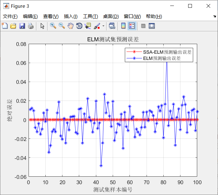
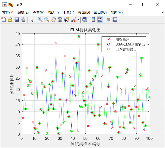
The prediction results are shown in the figure below

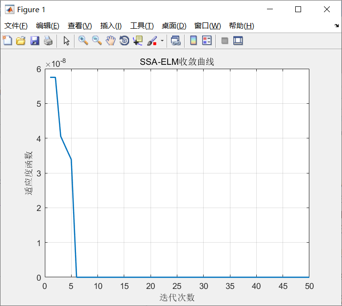
Error curve:

If you like, you can pay attention to me