Part III modeling and model evaluation

In the first two parts, we have processed the data of the Titanic. Interested partners can take a look at the first two articles. This article mainly introduces the third part of prediction analysis, that is, modeling and model evaluation. After data processing, let's see which model has the highest prediction accuracy under the condition of default parameters? No more nonsense, just open the code.

[note] data set downloads and project links can be obtained in official account [small white dragon] private letters, or in the whale community. Prediction and analysis of Titanic passenger survival in a classic case ]OK!! Or send me a private message directly in the background. When I see it, I will send Baidu online disk link ha!!

 

1. Data separation

The data processed by feature engineering is divided into initial training data and test data;

1.1 reading data

import pandas as pd
train = pd.read_csv('/home/mw/input/wlong9812/train.csv')
test = pd.read_csv('/home/mw/input/wlong9812/test.csv')
truth = pd.read_csv('/home/mw/input/wlong9812/gender_submission.csv')
train_and_test = pd.read_csv('/home/mw/input/wlong9812/Data processed by feature Engineering.csv')
PassengerId = test['PassengerId']

1.2 division of training set and test set

index = PassengerId[0] - 1
train_and_test_drop = train_and_test.drop(['PassengerId', 'Name', 'Ticket'], axis=1)
train_data = train_and_test_drop[:index]
test_data = train_and_test_drop[index:]

train_X = train_data.drop(['Survived'], axis=1)
train_y = train_data['Survived']
test_X = test_data.drop(['Survived'], axis=1)
test_y = truth['Survived']
train_X.shape, train_y.shape, test_X.shape

Note: the following models are modeled with default parameters, which do not involve too many parameter tuning, cross validation, complex models, etc. the main purpose is to compare the differences between different models with default parameters;

2. Modeling and model evaluation

This small chapter mainly implements the modeling and model evaluation part. For simplicity, the ready-made functions of sklearn are directly called. All models adopt default parameters and do not involve too many complex processes such as parameter optimization and algorithm optimization. Due to limited capacity, only some common basic models and integrated models are listed here. As for other models, readers can consult and supplement them by themselves; For slightly complex modeling such as algorithm optimization, we look forward to subsequent updates. We are making preparations... ヾ (≥ ▽≤ *) o

from sklearn.linear_model import LogisticRegression #Logistic regression
from sklearn.ensemble import RandomForestClassifier #Random forest
from sklearn.svm import SVC #Support vector machine
from sklearn.neighbors import KNeighborsClassifier #K nearest neighbor
from sklearn.tree import DecisionTreeClassifier #Decision tree
from sklearn.ensemble import GradientBoostingClassifier #Gradient lifting tree GBDT
import lightgbm as lgb #LightGBM algorithm
from xgboost.sklearn import XGBClassifier #XGBoost algorithm
from sklearn.ensemble import ExtraTreesClassifier #Extreme random tree
from sklearn.ensemble import AdaBoostClassifier # 
from sklearn.ensemble import BaggingClassifier

from sklearn.metrics import roc_auc_score #Accuracy evaluation model
import warnings
warnings.filterwarnings("ignore")

2.1 logistic regression

lr = LogisticRegression() #Logistic regression
lr.fit(train_X, train_y)
pred_lr = lr.predict(test_X) 
accuracy_lr = roc_auc_score(test_y, pred_lr)
print("Prediction results of logistic regression:", accuracy_lr)

2.2 random forest RF

rfc = RandomForestClassifier()
rfc.fit(train_X, train_y)
pred_rfc = rfc.predict(test_X)
accuracy_rfc = roc_auc_score(test_y, pred_rfc) 
print("Prediction results of random forest:", accuracy_rfc)

2.3 support vector machine SVM

svm = SVC()
svm.fit(train_X,train_y)
pred_svm = svm.predict(test_X)
accuracy_svm = roc_auc_score(test_y, pred_svm) 
print("Prediction results of support vector machine:", accuracy_svm)

2.4 K nearest neighbor KNN

knn = KNeighborsClassifier()
knn.fit(train_X,train_y)
pred_knn = knn.predict(test_X)
accuracy_knn = roc_auc_score(test_y, pred_knn) 
print("K Prediction results of nearest neighbor classifier:", accuracy_knn)

2.5 decision tree

dtree = DecisionTreeClassifier()
dtree.fit(train_X,train_y)
pred_dtree = dtree.predict(test_X)
accuracy_dtree = roc_auc_score(test_y, pred_dtree) 
print("Prediction results of decision tree model:", accuracy_dtree)

2.6 gradient lifting decision tree GBDT

gbdt = GradientBoostingClassifier()
gbdt.fit(train_X, train_y)
pred_gbdt = gbdt.predict(test_X)
accuracy_gbdt = roc_auc_score(test_y, pred_gbdt) 
print("GBDT Prediction results of the model:", accuracy_gbdt)

2.7 LightGBM algorithm

lgb_train = lgb.Dataset(train_X, train_y)
lgb_eval = lgb.Dataset(test_X, test_y, reference = lgb_train)

gbm = lgb.train(params = {}, train_set = lgb_train, valid_sets = lgb_eval)
pred_lgb = gbm.predict(test_X, num_iteration = gbm.best_iteration)
accuracy_lgb = roc_auc_score(test_y, pred_lgb) 
print("LightGBM Prediction results of the model:", accuracy_lgb)

2.8 XGBoost algorithm

xgbc = XGBClassifier()
xgbc.fit(train_X, train_y)
pred_xgbc = xgbc.predict(test_X)
accuracy_xgbc = roc_auc_score(test_y, pred_xgbc) 
print("XGBoost Prediction results of the model:", accuracy_xgbc)

2.9 extreme random tree

etree = ExtraTreesClassifier()
etree.fit(train_X, train_y)
pred_etree = etree.predict(test_X)
accuracy_etree = roc_auc_score(test_y, pred_etree)
print("Prediction results of extreme random tree model:", accuracy_etree)

2.10 AdaBoost algorithm

abc = AdaBoostClassifier()
abc.fit(train_X, train_y)
pred_abc = abc.predict(test_X)
accuracy_abc = roc_auc_score(test_y, pred_abc) 
print("AdaBoost Prediction results of the model:", accuracy_abc)

2.11 K-nearest neighbor based on Bagging

bag_knn = BaggingClassifier(KNeighborsClassifier())
bag_knn.fit(train_X, train_y)
pred_bag_knn = bag_knn.predict(test_X)
accuracy_bag_knn = roc_auc_score(test_y, pred_bag_knn)
print("be based on Bagging of K Prediction results of the nearest neighbor model:", accuracy_bag_knn)

2.12 decision tree based on Bagging

bag_dt = BaggingClassifier(DecisionTreeClassifier())
bag_dt.fit(train_X, train_y)
pred_bag_dt = bag_dt.predict(test_X)
accuracy_bag_dt = roc_auc_score(test_y, pred_bag_dt)
print("be based on Bagging Prediction results of decision tree model:", accuracy_bag_dt)

3. Summary

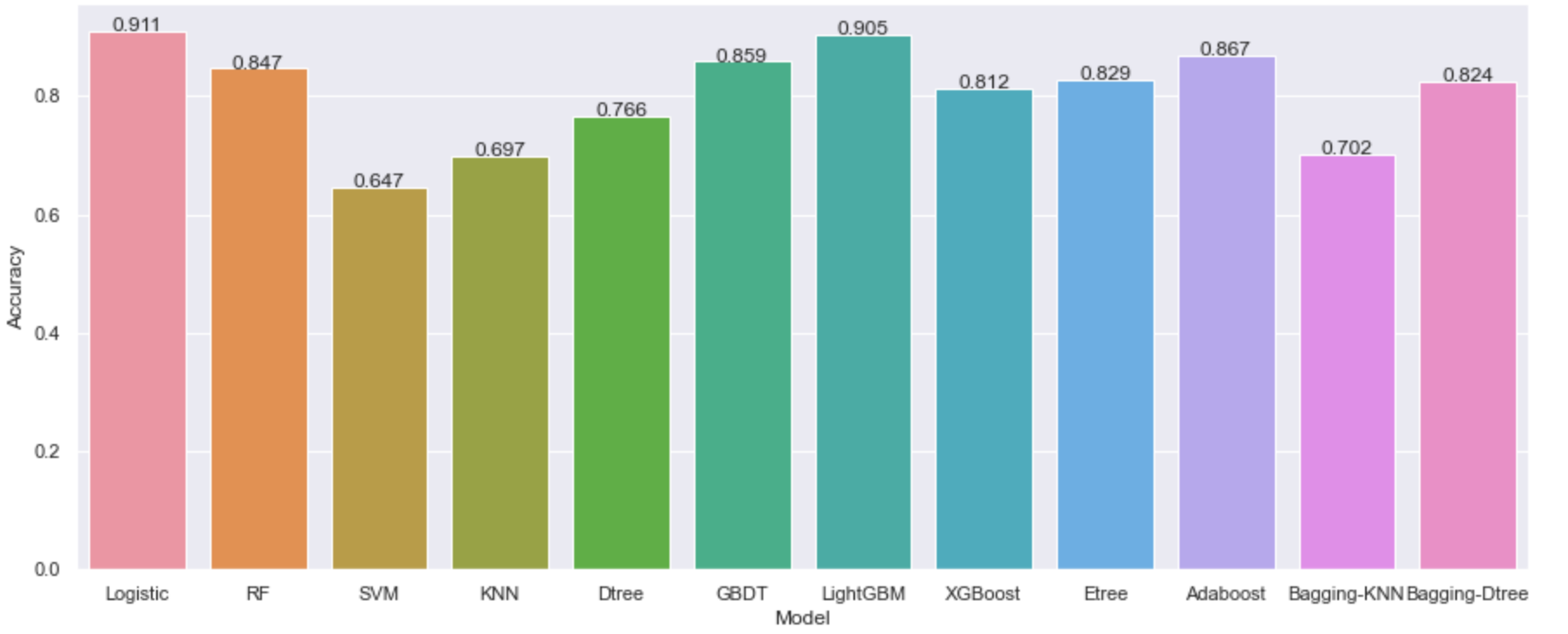
import seaborn as sns
import matplotlib.pyplot as plt

sns.set(rc={'figure.figsize':(15,6)}) #Set canvas size
accuracys = [accuracy_lr, accuracy_rfc, accuracy_svm, accuracy_knn, accuracy_dtree, accuracy_gbdt, accuracy_lgb,accuracy_xgbc, accuracy_etree, accuracy_abc, accuracy_bag_knn, accuracy_bag_dt, ]
models = ['Logistic', 'RF', 'SVM', 'KNN', 'Dtree', 'GBDT', 'LightGBM', 'XGBoost', 'Etree', 'Adaboost', 'Bagging-KNN', 'Bagging-Dtree']
bar = sns.barplot(x=models, y=accuracys)

#Display value label
for x, y in enumerate(accuracys):
    plt.text(x, y, '%s'% round(y,3), ha='center')

plt.xlabel("Model")
plt.ylabel("Accuracy")
plt.show()

According to the above bar chart, under the condition of all model default parameters, the prediction accuracy of logistic regression is the highest, reaching 0.911, followed by LightGBM model, which is also above 0.9. The models with an accuracy of more than 80% include RF, GBDT, XGBoost, ETree, Adaboost and decision tree based on Bagging, while the prediction accuracy of other models is lower;

Since the models involved in this paper have not been optimized by algorithm, we can only simply see the comparison of prediction accuracy between models under default parameters, but the above results do not represent the upper limit of prediction accuracy of each model. For example, some models have low accuracy under default parameters, but may become very high through parameter adjustment and algorithm optimization. This small chapter is mainly for beginners to have a basic understanding of algorithm prediction and learn to use it simply. As for the subsequent algorithm optimization, look forward to the subsequent updates!