R language implementation COPULA algorithm modeling dependency case analysis report

Original link: http://tecdat.cn/?p=6193

Original source: Tuo end data tribal official account

Copula is a function that couples multivariable distribution function with its edge distribution function, which is usually called edge. Copula is an excellent tool for modeling and simulating related random variables. The main attraction of Copula is that by using them, you can model the relevant structures and edges (i.e. the distribution of each random variable) respectively.

How copulas work

First, let's understand how copula works.

 set.seed(100)

m < -  3
n < -  2000
 
z < -  mvrnorm(n，mu = rep(0，m)，Sigma = sigma，empirical = T)

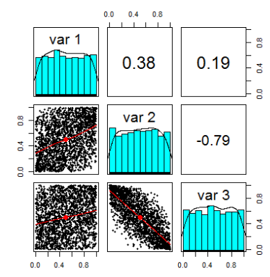
We use cor() and scatter matrix to check the sample correlation.

 pairs.panels(Z)

          \[，1\] \[，2\] \[，3\]
\[1，\] 1.0000000 0.3812244 0.1937548
\[2，\] 0.3812244 1.0000000 -0.7890814
\[3，\] 0.1937548 -0.7890814 1.0000000

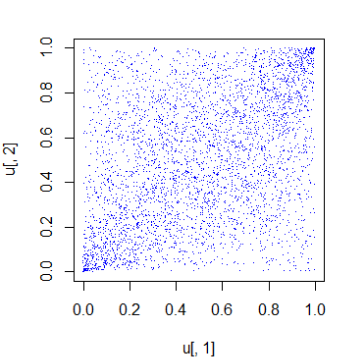
 pairs.panels(U)

This is a scatter matrix u with new random variables.

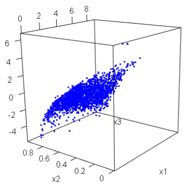
We can draw a 3D graph of a vector to represent u.

Now, as a final step, we just need to select the edge and apply it. I selected edges for Gamma, Beta and Student and used the parameters specified below.

x1 < -  qgamma(u \[，1\]，shape = 2，scale = 1)
x2 < -  qbeta(u \[，2\]，2,2)
x3 < -  qt(u \[，3\]，df = 5)

The following is a 3D graph of our simulated data.

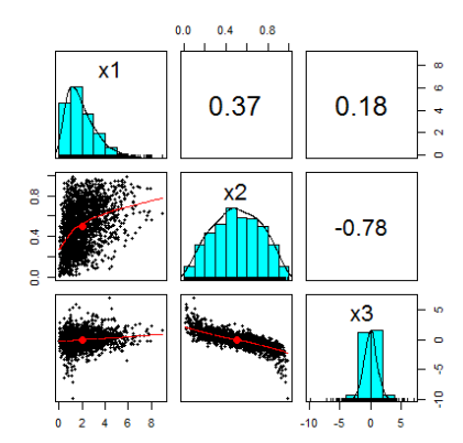
df < -  cbind(x1，x2，x3)
pairs.panels(DF)
 
          x1 x2 x3
x1 1.0000000 0.3812244 0.1937548
x2 0.3812244 1.0000000 -0.7890814
x3 0.1937548 -0.7890814 1.0000000

This is the scatter matrix of random variables:

Using copula

Let's use copula to copy the above process.

Now that we have specified the dependency structure and set the edge through copula (ordinary copula), the mvdc() function generates the required distribution. Then we can use the rmvdc() function to generate random samples.

 colnames(Z2)< -  c("x1"，"x2"，"x3")
pairs.panels(Z2)

Of course, the simulation data is very close to the previous data and is displayed in the following scatter diagram matrix:

Simple application example

Now for the real world example. We will fit two stocks and try to use copula simulation.

Let's load in R:

cree < -  read.csv('cree_r.csv'，header = F)$ V2
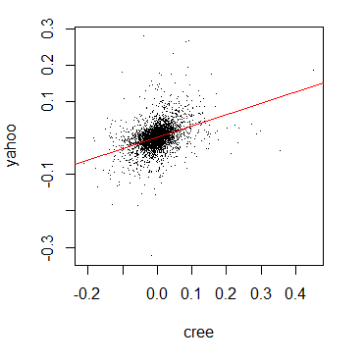
yahoo < -  read.csv('yahoo_r.csv'，header = F)$ V2

Before going directly to the copula fitting process, let's check the correlation between the returns of the two stocks and draw the regression line:

We can see a positive correlation:

In the first example above, I chose a normal copula model, but when applying these models to actual data, we should carefully consider which models are more suitable for the data. For example, many copulas are more suitable for modeling asymmetric correlation, others emphasize tail correlation, and so on. My guess about stock returns is that t-copula should be OK, but guess is definitely not enough. Essentially, it allows us to perform copula selection using BIC and AIC through functions:

 
  pobs(as.matrix(cbind(cree，yahoo)))\[，1\]
  selectedCopula
 

$ PAR
\[1\] 0.4356302

$ PAR2
\[1\] 3.844534

The fitting algorithm does choose t-copula and estimates the parameters for us.
Let's try to fit the proposed model and check the parameter fitting.

t.cop  
set.seed(500)
m < -  pobs(as.matrix(cbind(cree，yahoo)))
 
COEF(FIT)

  rho.1 df 
0.43563 3.84453

Let's look at the density of copula we just estimated

rho < -  coef(fit)\[1\]
df < -  coef(fit)\[2\]

Now we just need to build Copula and take 3965 random samples from it.

  rCopula(3965，tCopula(  = 2， ，df = df))
 

          \[，1\] \[，2\]
\[1，\] 1.0000000 0.3972454
\[2，\] 0.3972454 1.0000000

This is a graph of the samples included:

t-copula is usually suitable for the phenomenon that there is a high correlation in the extreme value (the tail of the distribution).
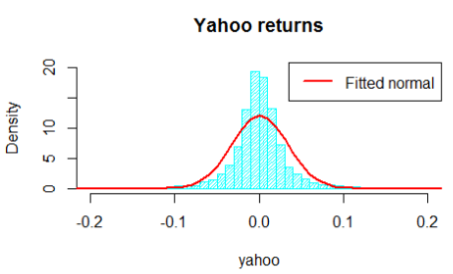
Now we face the difficulty: modeling the edges. For simplicity, we will assume a normal distribution. Therefore, we estimate the parameters of the edge.

The histogram is shown as follows:

Now we apply copula in the function to obtain the simulated observations from the generated multivariable distribution. Finally, we compare the simulation results with the original data.

This is the final scatter diagram of the data under the assumption of normal distribution edge and t-copula of dependent structure:

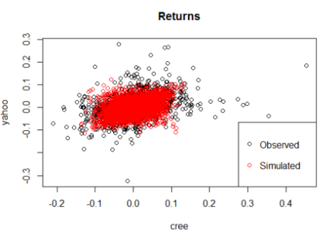
As you can see, t-copula causes the results to be close to the actual observations.

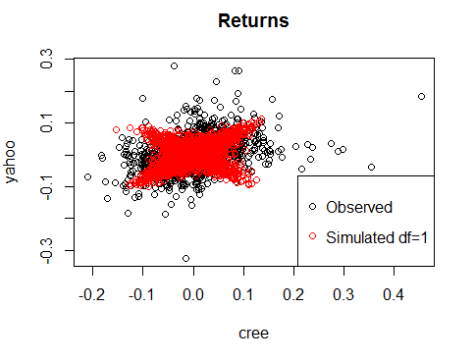
Let's try df=1 and df=8:

Obviously, this parameter df is very important for determining the shape of the distribution. With the increase of df, t-copula tends to be normally distributed copula.