Exploration of K-means clustering algorithm

import  numpy as np
import matplotlib.pyplot as plt
import sklearn.datasets as ds
import matplotlib.colors
from sklearn.cluster import  KMeans,MiniBatchKMeans

def expand(a,b):
    d=(b-a)*0.1
    return a-d,b+d
if __name__ == '__main__':
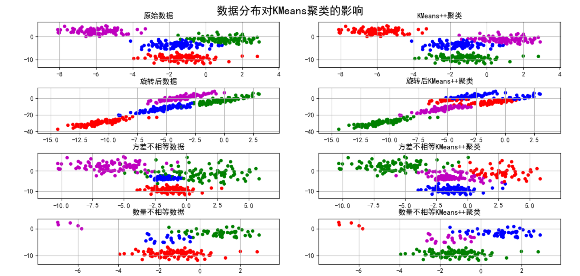
    N=400               #Create 400 samples
    centers=4           #Create 4 sets of data
    # n_features=2 samples contain 2 dimension centers, so the samples are distributed in 4 clusters
    # The return value data, y, means that we created the data through ds. In fact, we know the data in that label
    data,y=ds.make_blobs(N,n_features=2,centers=centers,random_state=2)
    # Specify the variance of the four groups to create data
    data2,y2 = ds.make_blobs(N, n_features=2, centers=centers,cluster_std=(1,2.5,0.5,2),random_state=2)
    #All the data of the first group of data, the second group of data to the top 50, the top 20 of the third group of data and the top 5 of the fourth group of data
    data3=np.vstack((data[y==0][:],data[y==1][:50],data[y==2][:20],data[y==3][:5]))
    # Label the data3 data
    y3=np.array([0]*100+[1]*50+[2]*20+[3]*5)
    #  Create KMeans object
    cls=KMeans(n_clusters=4,init='k-means++')  #initial
    y_hat=cls.fit_predict(data)  #Training and prediction data
    y2_hat = cls.fit_predict(data2) #Training and prediction data2
    y3_hat = cls.fit_predict(data3) #Training and prediction data3

    m=np.array(((1,1),(1,3)))  #Create a matrix
    data_r=data.dot(m)         #Use the created matrix to linearly transform data
    y_r_hat=cls.fit_predict(data_r)  #Training and prediction data_r
    matplotlib.rcParams['font.sans-serif']=[u'SimHei'] #Can display Chinese
    matplotlib.rcParams['axes.unicode_minus'] = False
    cm=matplotlib.colors.ListedColormap(list('rgbm'))
    plt.figure(figsize=(9,10),facecolor='w')
    plt.subplot(421)
    plt.title(u'raw data')
    plt.scatter(data[:,0],data[:,1],c=y,s=30,cmap=cm,edgecolors='none')
    x1_min, x2_min = np.min(data, axis=0)
    x1_max, x2_max = np.max(data, axis=0)
    x1_min, x1_max = expand(x1_min, x1_max)
    x2_min, x2_max = expand(x2_min, x2_max)
    plt.xlim((x1_min, x1_max))
    plt.ylim((x2_min, x2_max))
    plt.grid(True)

    plt.subplot(422)
    plt.title(u'KMeans++clustering')
    plt.scatter(data[:, 0], data[:, 1], c=y_hat, s=30, cmap=cm, edgecolors='none')
    plt.xlim((x1_min, x1_max))
    plt.ylim((x2_min, x2_max))
    plt.grid(True)

    plt.subplot(423)
    plt.title(u'Data after rotation')
    plt.scatter(data_r[:, 0], data_r[:, 1], c=y, s=30, cmap=cm, edgecolors='none')
    x1_min, x2_min = np.min(data_r, axis=0)
    x1_max, x2_max = np.max(data_r, axis=0)
    x1_min, x1_max = expand(x1_min, x1_max)
    x2_min, x2_max = expand(x2_min, x2_max)
    plt.xlim((x1_min, x1_max))
    plt.ylim((x2_min, x2_max))
    plt.grid(True)

    plt.subplot(424)
    plt.title(u'After rotation KMeans++clustering')
    plt.scatter(data_r[:, 0], data_r[:, 1], c=y_r_hat, s=30, cmap=cm, edgecolors='none')
    plt.xlim((x1_min, x1_max))
    plt.ylim((x2_min, x2_max))
    plt.grid(True)

    plt.subplot(425)
    plt.title(u'Unequal variance data')
    plt.scatter(data2[:, 0], data2[:, 1], c=y2, s=30, cmap=cm, edgecolors='none')
    x1_min, x2_min = np.min(data2, axis=0)
    x1_max, x2_max = np.max(data2, axis=0)
    x1_min, x1_max = expand(x1_min, x1_max)
    x2_min, x2_max = expand(x2_min, x2_max)
    plt.xlim((x1_min, x1_max))
    plt.ylim((x2_min, x2_max))
    plt.grid(True)

    plt.subplot(426)
    plt.title(u'Unequal variance KMeans++clustering')
    plt.scatter(data2[:, 0], data2[:, 1], c=y2_hat, s=30, cmap=cm, edgecolors='none')
    plt.xlim((x1_min, x1_max))
    plt.ylim((x2_min, x2_max))
    plt.grid(True)

    plt.subplot(427)
    plt.title(u'Unequal quantity data')
    plt.scatter(data3[:, 0], data3[:, 1], s=30, c=y3, cmap=cm, edgecolors='none')
    x1_min, x2_min = np.min(data3, axis=0)
    x1_max, x2_max = np.max(data3, axis=0)
    x1_min, x1_max = expand(x1_min, x1_max)
    x2_min, x2_max = expand(x2_min, x2_max)
    plt.xlim((x1_min, x1_max))
    plt.ylim((x2_min, x2_max))
    plt.grid(True)

    plt.subplot(428)
    plt.title(u'Unequal quantity KMeans++clustering')
    plt.scatter(data3[:, 0], data3[:, 1], c=y3_hat, s=30, cmap=cm, edgecolors='none')
    plt.xlim((x1_min, x1_max))
    plt.ylim((x2_min, x2_max))
    plt.grid(True)

    plt.tight_layout(2, rect=(0, 0, 1, 0.97))
    plt.suptitle(u'Data distribution pair KMeans Influence of clustering', fontsize=18)
    # https://github.com/matplotlib/matplotlib/issues/829
    # plt.subplots_adjust(top=0.92)
    plt.show()
    # plt.savefig('cluster_kmeans')

Exploration of relevant indicators

# !/usr/bin/python
# -*- coding:utf-8 -*-

from sklearn import metrics


if __name__ == "__main__":
    y = [0, 0, 0, 1, 1, 1]
    y_hat = [0, 0, 1, 1, 2, 2]
    h = metrics.homogeneity_score(y, y_hat)
    c = metrics.completeness_score(y, y_hat)
    print(u'identity(Homogeneity): ', h)
    print(u'Integrity(Completeness): ', c)
    v2 = 2 * c * h / (c + h)
    v = metrics.v_measure_score(y, y_hat)
    print(u'V-Measure: ', v2, v)

    y = [0, 0, 0, 1, 1, 1]
    y_hat = [0, 0, 1, 3, 3, 3]
    h = metrics.homogeneity_score(y, y_hat)
    c = metrics.completeness_score(y, y_hat)
    v = metrics.v_measure_score(y, y_hat)
    print(u'identity(Homogeneity): ', h)
    print(u'Integrity(Completeness): ', c)
    print(u'V-Measure: ', v)

    # Allow different values
    y = [0, 0, 0, 1, 1, 1]
    y_hat = [1, 1, 1, 0, 0, 0]
    h = metrics.homogeneity_score(y, y_hat)
    c = metrics.completeness_score(y, y_hat)
    v = metrics.v_measure_score(y, y_hat)
    print(u'identity(Homogeneity): ', h)
    print(u'Integrity(Completeness): ', c)
    print(u'V-Measure: ', v)

    y = [0, 0, 1, 1]
    y_hat = [0, 1, 0, 1]
    ari = metrics.adjusted_rand_score(y, y_hat)
    print(ari)

    y = [0, 0, 0, 1, 1, 1]
    y_hat = [0, 0, 1, 1, 2, 2]
    ari = metrics.adjusted_rand_score(y, y_hat)
    print(ari)

result

identity(Homogeneity):  0.6666666666666669
 Integrity(Completeness):  0.420619835714305
V-Measure:  0.5158037429793889 0.5158037429793889
 identity(Homogeneity):  1.0
 Integrity(Completeness):  0.6853314789615865
V-Measure:  0.8132898335036762
 identity(Homogeneity):  1.0
 Integrity(Completeness):  1.0
V-Measure:  1.0
-0.5
0.24242424242424243

Process finished with exit code 0

hierarchical clustering

Splitting method

• 1. Group all samples into one cluster

• While does not meet the condition (k number or distance threshold):

• calculate the distance between samples in the same cluster C, and select the two samples ab with the farthest distance (termination condition detection)

• classify samples a and b into C1 and C2 (termination condition test)

• calculate who the sample in cluster c is close to and into

 

Coagulation method

• While does not meet the conditions:

• calculate the distance between two clusters and find the cluster C1 and C2 with the minimum distance (multiple calculation methods)

• merge C1 and C2

        

• how to combine C1 and C2:

        • 1. The sample distance with the smallest distance between two clusters

• 1 2The distance between the two farthest points of two clusters

        • 3. Draw the distance between two clusters

        • 4. The median of the distance between two thick

        • 5. Find the center point of each set, and the distance of the center point represents the distance of the cluster

Hierarchical clustering contrast k-means

        

Density clustering DBSCAN

 

• DBSCAN(Density-Based Spatial Clustering of Applications　with Noise)

 

• an algorithm based on density clustering, which is different from hierarchical clustering. It defines clusters as the largest set of points connected by density, can divide regions with high density into clusters, and can effectively resist noise

Q: define cluster as the largest set of points connected by density?

Concept 1: direct density up to:

• e neighborhood of object: the area of a given object within radius E;

• core object: given a number m, if there are at least m objects in the e neighborhood of the object,

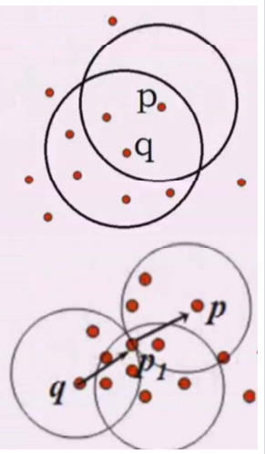
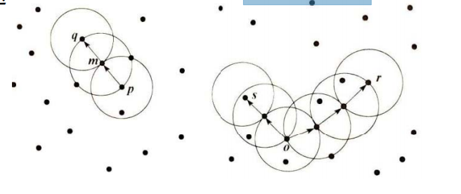
This object is the core object

• direct density up to: given an object set D, If p is in the e neighborhood of q and q is a core object, p starts from q

The starting point is directly accessible

• density reachability: if there is an object chain p1p2... pn, so that p1=p,pn=q,pi+1 is directly density reachable with respect to e and m, then object P is density reachable with respect to e and m from object Q.

• density connection: if there is an object o in set D, the density of O - > P can reach, O - > Q If the density can be reached, then p and q are related to the density of e and m

 

DB SCAN algorithm

• DB-SCAN looks for clusters by examining the e-neighborhood of each object in the dataset

•

If there is more than m in the e neighborhood of a point p Create a new object with p as the core Cluster, repeatedly search for density connected sets according to p (it is possible to merge the original generated clusters). When no new points can be added to the cluster, the search ends.

DB_SCAN exploration

# !/usr/bin/python
# -*- coding:utf-8 -*-

import numpy as np
import matplotlib.pyplot as plt
import sklearn.datasets as ds
import matplotlib.colors
from sklearn.cluster import DBSCAN
from sklearn.preprocessing import StandardScaler


def expand(a, b):
    d = (b - a) * 0.1
    return a-d, b+d


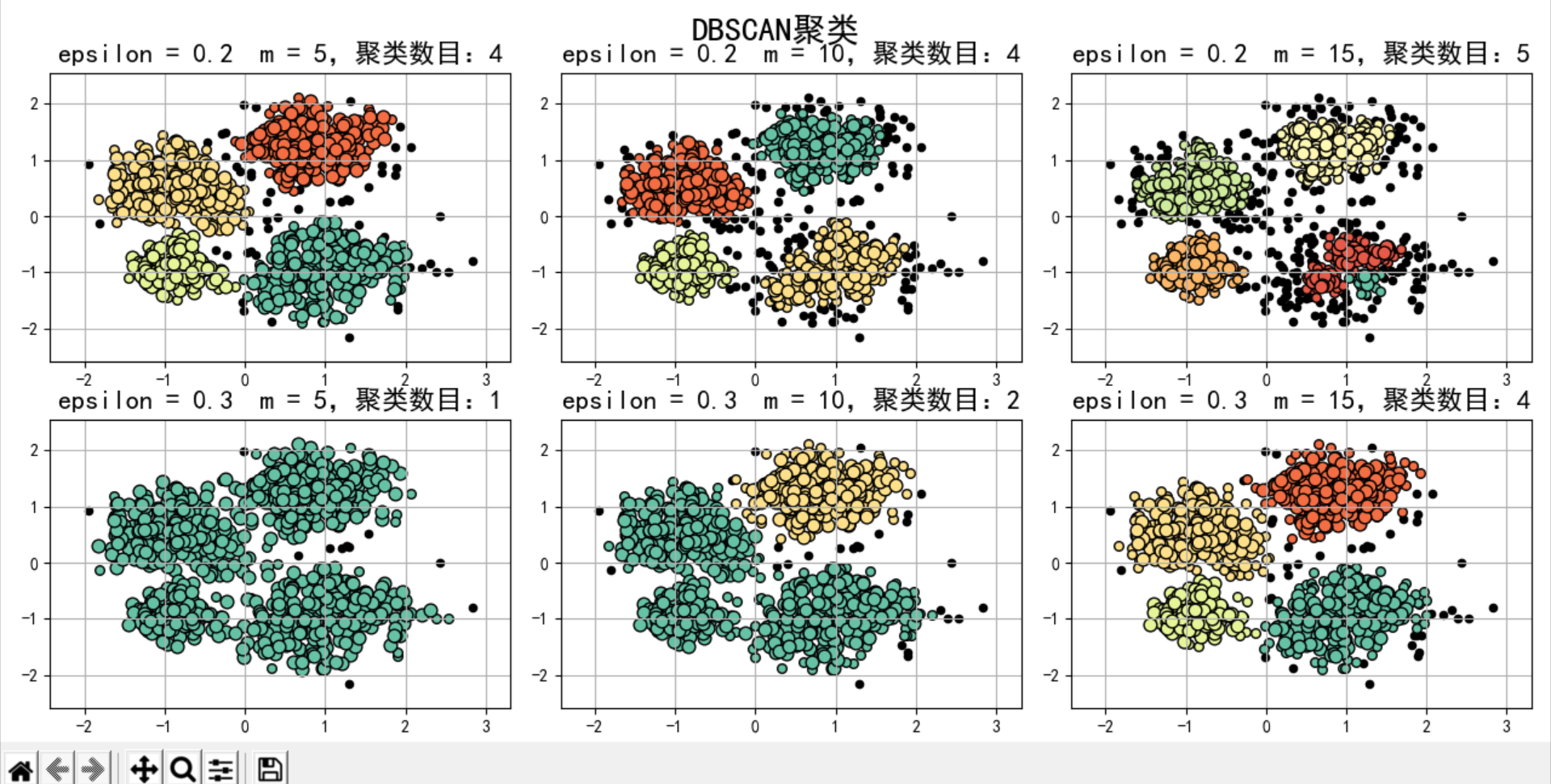
if __name__ == "__main__":
    N = 1000
    centers = [[1, 2], [-1, -1], [1, -1], [-1, 1]]
    data, y = ds.make_blobs(N, n_features=2, centers=centers, cluster_std=[0.5, 0.25, 0.7, 0.5], random_state=0)
    data = StandardScaler().fit_transform(data)
    # Parameters of data:(epsilon, min_sample)  #epsilon radius min_ The minimum number of samples in the radius of sample is used to judge whether it is a core object
    params = ((0.2, 5), (0.2, 10), (0.2, 15), (0.3, 5), (0.3, 10), (0.3, 15))

    matplotlib.rcParams['font.sans-serif'] = [u'SimHei']
    matplotlib.rcParams['axes.unicode_minus'] = False

    plt.figure(figsize=(12, 8), facecolor='w')
    plt.suptitle(u'DBSCAN clustering', fontsize=20)

    for i in range(6):
        eps, min_samples = params[i]
        model = DBSCAN(eps=eps, min_samples=min_samples)
        model.fit(data)
        y_hat = model.labels_

        core_indices = np.zeros_like(y_hat, dtype=bool)
        core_indices[model.core_sample_indices_] = True

        y_unique = np.unique(y_hat)
        n_clusters = y_unique.size - (1 if -1 in y_hat else 0)
        print(y_unique, 'The number of clusters is:', n_clusters)

        plt.subplot(2, 3, i+1)
        clrs = plt.cm.Spectral(np.linspace(0, 0.8, y_unique.size))
        print(clrs)
        for k, clr in zip(y_unique, clrs):
            cur = (y_hat == k)
            if k == -1:
                plt.scatter(data[cur, 0], data[cur, 1], s=20, c='k')
                continue
            plt.scatter(data[cur, 0], data[cur, 1], s=30, c=clr, edgecolors='k')
            plt.scatter(data[cur & core_indices][:, 0], data[cur & core_indices][:, 1], s=60, c=clr, marker='o', edgecolors='k')
        x1_min, x2_min = np.min(data, axis=0)
        x1_max, x2_max = np.max(data, axis=0)
        x1_min, x1_max = expand(x1_min, x1_max)
        x2_min, x2_max = expand(x2_min, x2_max)
        plt.xlim((x1_min, x1_max))
        plt.ylim((x2_min, x2_max))
        plt.grid(True)
        plt.title(u'epsilon = %.1f  m = %d，Number of clusters:%d' % (eps, min_samples, n_clusters), fontsize=16)
    plt.tight_layout()
    plt.subplots_adjust(top=0.9)
    plt.show()