1, Gray histogram

Concept:

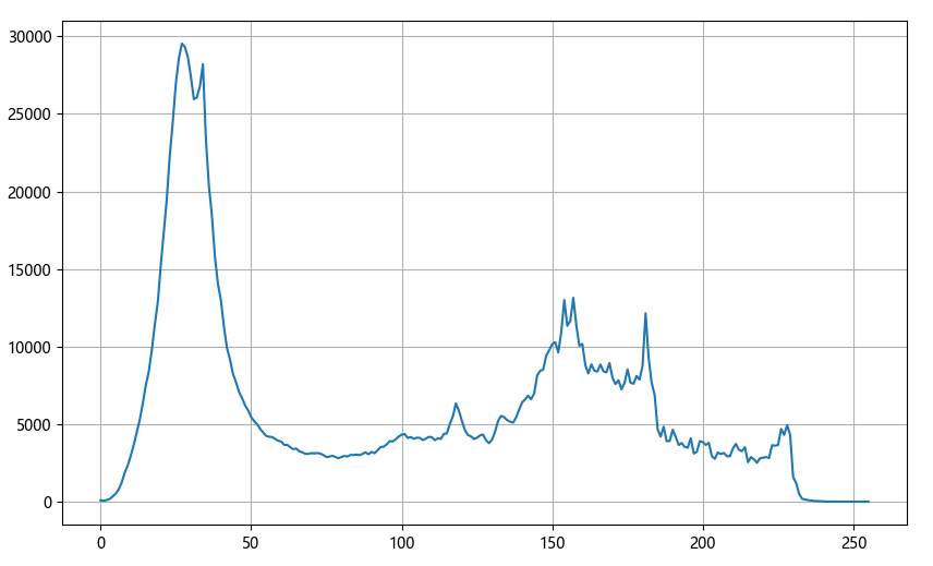
Image histogram is a histogram representing the brightness distribution in a digital image. It plots the number of pixels of each brightness value in the image.

In this histogram, the left side of the abscissa is a darker area and the right side is a brighter area. Therefore, the data in the histogram of a darker image is mostly concentrated in the left and middle parts, while the image with overall brightness and only a small amount of shadow is the opposite. As shown in the figure:

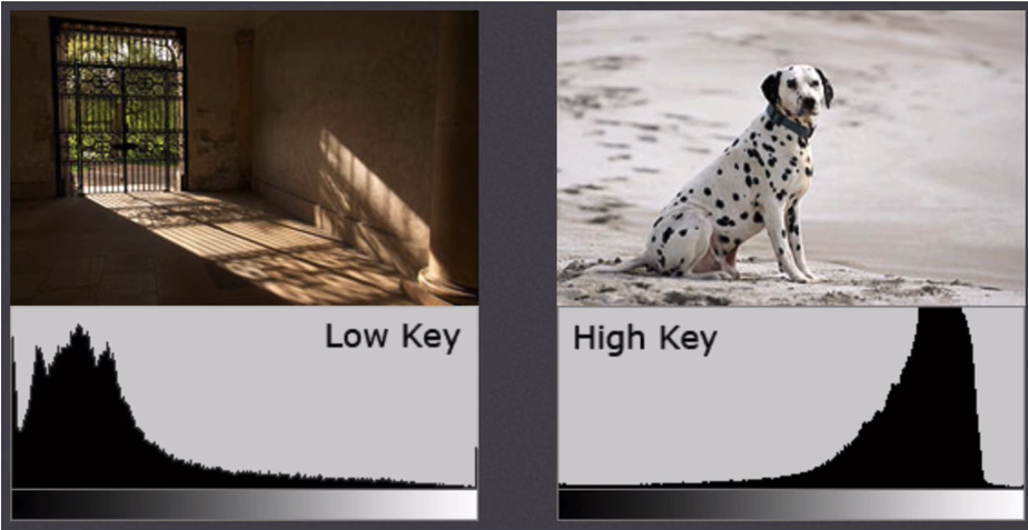
Note: the image histogram is drawn according to the gray image, not the color image.

Terms of image histogram:

1. dims: the number of features to be counted.
   (for example, if only gray values are counted, dims=1; if BGR three colors are counted, dims=3)
2. bins: the number of sub segments in each feature space.
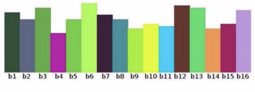
   (as shown in the histogram in the figure below, if each vertical bar represents a certain value or an interval, the bins of the histogram = 16)
3. Range: the value range of the feature to be counted.
   (as shown in the figure below, we divide the [0255] interval into 16 sub intervals, where range = [0255])

Significance of histogram:

Histogram is a graphical representation of pixel intensity distribution in an image.

It counts the number of pixels for each intensity value.

The histograms of different images may be the same

OpenCv API:

cv2.calcHist(images, channels, mask, histSize, ranges)

Parameters:

1. images: original image. When a function is passed in, it should be enclosed by brackets [], for example: [img]
2. Channels: if the input image is a grayscale image, its value is [0]; If it is a color image, the input parameters can be [0], [1], [2], which correspond to channels B, G and R respectively.
3. Mask: mask image. To count the histogram of the whole image, set it to None. But if you want to count the histogram of a part of the image, you need to make a mask image and use it.
4. histSize: number of bins. It should also be enclosed in square brackets, for example: [256].
5. ranges: range of pixel values. Usually [0256].

Coding:

import cv2 as cv
import matplotlib.pyplot as plt

src = cv.imread("E:\\view.jpg", 0)  # Read directly in grayscale image
img = src.copy()

# Statistical grayscale image
greyScale_map = cv.calcHist([img], [0], None, [256], [0, 256])

# Draw grayscale image
plt.figure(figsize=(10, 6), dpi=100)
plt.plot(greyScale_map)
plt.grid()
plt.show()

   

II. Application of mask

Principle:

Mask is to block the image to be processed with the selected image, figure or object to control the area of image processing.
In digital image processing, we usually use two-dimensional matrix array for mask. The mask is a binary image composed of 0 and 1. The mask image is used to mask the image to be processed, in which the 1 value area is processed, and the 0 value area is shielded and will not be processed.
Application:

The main uses of the mask are:

1. Extracting region of interest: perform "and" operations with the pre-made region of interest mask and the image to be processed to obtain the region of interest image. The image value in the region of interest remains unchanged, while the image value outside the region of interest is 0.
2. Shielding function: mask some areas on the image so that they do not participate in the processing or the calculation of processing parameters, or only process or count the shielding area.
3. Structural feature extraction: detect and extract the structural features similar to the mask in the image by similarity variable or image matching method·
4. Special shape image making.

Mask is widely used in remote sensing image processing. When extracting roads, rivers or houses, a mask matrix is used to filter the pixels of the image, and then the features or signs we need are highlighted.

Coding:

import cv2 as cv
import matplotlib.pyplot as plt
import numpy as np

src = cv.imread("E:\\view.jpg", 0)  # Read directly in grayscale image
img = src.copy()

# Create mask
mask = np.zeros(img.shape[:2], np.uint8)
mask[700:1000, 100:400] = 1

# Mask
masked_img = cv.bitwise_and(img, img, mask=mask)  # And operation

# Gray level image after statistical mask
mask_histr = cv.calcHist([img], [0], mask, [256], [0, 256])

# Display image
fig, axes = plt.subplots(nrows=2, ncols=2, figsize=(10, 8), dpi=100)
axes[0][0].imshow(img, cmap=plt.cm.gray)
axes[0][0].set_title("Original drawing")
axes[0][1].imshow(mask, cmap=plt.cm.gray)
axes[0][1].set_title("Mask data")
axes[1][0].imshow(masked_img, cmap=plt.cm.gray)
axes[1][0].set_title("Post mask image")
axes[1][1].plot(mask_histr)
axes[1][1].grid()
axes[1][1].set_title("Gray histogram of image after mask")
plt.show()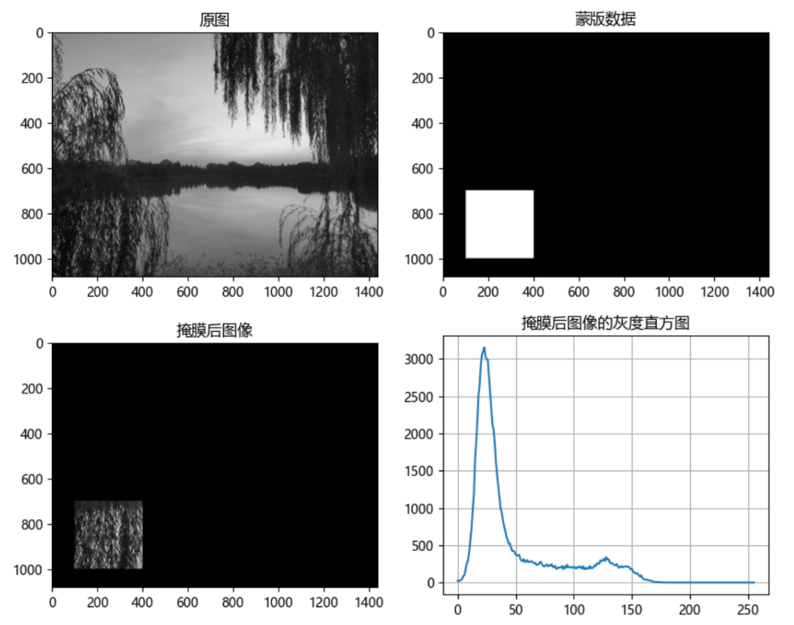

3, Histogram equalization

Principle:

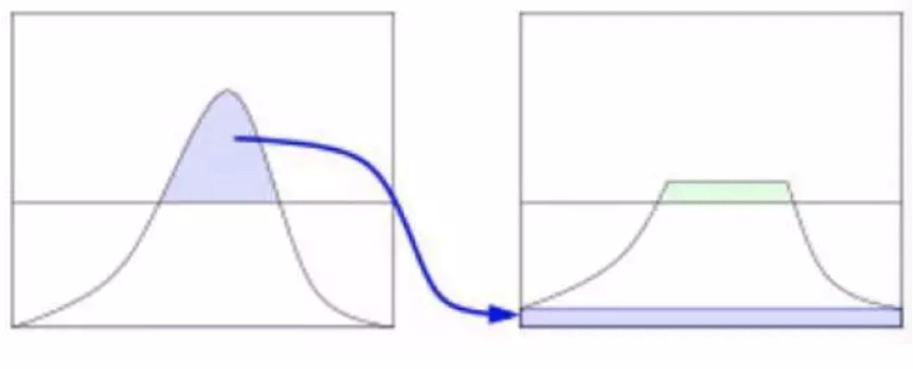
Imagine if the pixel values of most pixels in an image are concentrated in a small gray value range? If an image is bright as a whole, the number of pixel values should be high. Therefore, its histogram should be stretched horizontally (as shown in the figure below), which can expand the distribution range of image pixel values and improve the image contrast. This is what histogram equalization should do.
 

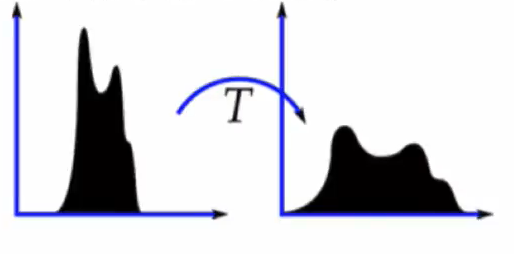
"Histogram equalization" is to change the gray histogram of the original image from a relatively concentrated gray range to a distribution in a wider gray range. Histogram equalization is to stretch the image nonlinearly and redistribute the image pixel values to make the number of pixels in a certain gray range roughly the same.

Application:

Improve the overall contrast of the image.

Especially when the pixel value distribution of useful data is close, it is widely used in X-ray images, which can improve the display of skeleton structure. In addition, it can better highlight details in overexposed or underexposed images.
 

 OpenCv API:

cv2.equalizeHist(img)

Parameters:

img: input grayscale image

Coding:

import cv2 as cv
import matplotlib.pyplot as plt
import numpy as np

src = cv.imread("E:\\qi.png", 0)  # Read directly in grayscale image
img = src.copy()

# Equalization treatment
dst = cv.equalizeHist(img)

# Display image
fig, axes = plt.subplots(nrows=1, ncols=2, figsize=(10, 8), dpi=100)
axes[0].imshow(img, cmap=plt.cm.gray)
axes[0].set_title("Original drawing")
axes[1].imshow(dst, cmap=plt.cm.gray)
axes[1].set_title("Equalized image")
plt.show()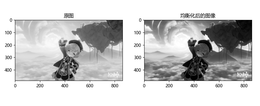

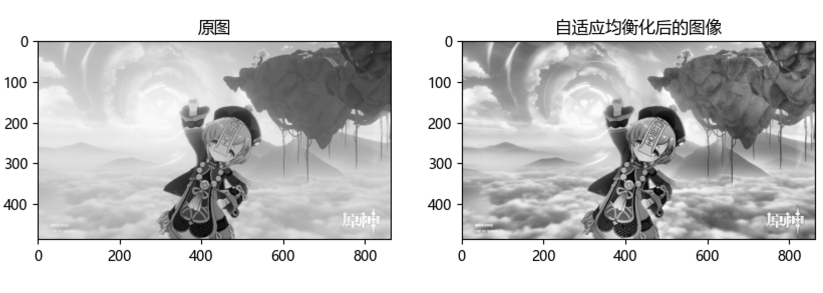
IV. adaptive histogram equalization

Origin:

In the above histogram equalization, we consider the global contrast of the image. Indeed, after histogram equalization, the contrast of the picture background is changed, but in many cases, the effect is not good, because the image after equalization is likely to be partially too bright or partially too dark, resulting in the loss of data information.
 

Principle:

1. Divide the whole image into many small blocks, which are called "tiles" (the default size of tiles in OpenCV is 8x8), and then perform histogram equalization for each small block. (therefore, in each region, the histogram will be concentrated in a small region).
2. If there is noise, the noise will be amplified. To avoid this, use contrast limits. For each small block, if the bin in the histogram exceeds the upper limit of contrast, the pixels in the histogram are evenly dispersed into other bins, and then histogram equalization is carried out.

   

3. Finally, in order to remove the boundary between each block, bilinear difference is used to splice each block.
    

OpenCv API:

clahe = cv.createCLAHE(clipLimit, tileGridSize)
dst = clahe.apply(img)

Parameters:

1. clipLimit: contrast limit. The default value is 40
2. tileGridSize: block size. The default value is 8 * 8

Coding:

import cv2 as cv
import matplotlib.pyplot as plt
import numpy as np

src = cv.imread("E:\\qi.png", 0)  # Read directly in grayscale image
img = src.copy()

# Create an adaptive equalization object and apply it to the image
clahe = cv.createCLAHE(clipLimit=3.0, tileGridSize=(8, 8))
dst = clahe.apply(img)

# Display image
fig, axes = plt.subplots(nrows=1, ncols=2, figsize=(10, 8), dpi=100)
axes[0].imshow(img, cmap=plt.cm.gray)
axes[0].set_title("Original drawing")
axes[1].imshow(dst, cmap=plt.cm.gray)
axes[1].set_title("Image after adaptive equalization")
plt.show()