**
1. What is a lookup table
**
In daily life, we have to do some searching work almost every day, looking up someone's phone number in the phone book; Find a specific file in the folder of the computer, and so on. This section mainly introduces the data structure used for lookup operation - lookup table.
A lookup table is a collection of data elements of the same type. For example, a telephone directory and a dictionary can be regarded as a look-up table.
Generally, there are several operations for lookup tables:
Find a specific data element in the lookup table;
Insert data elements into the lookup table;
Delete data elements from the lookup table;
Static lookup table and dynamic lookup table
In the lookup table, only the lookup operation is performed without changing the data elements in the table. This kind of lookup table is called static lookup table; On the contrary, the operation of inserting or deleting data while performing the lookup operation in the lookup table is called dynamic lookup table.
keyword
When looking up a specific element in the lookup table, the premise is to know some attributes of the element. For example, everyone will have their own unique student number when they go to school, because your name and age may be repeated with others, but the student number will not be repeated. These attributes of students (student number, name, age, etc.) can be called keywords.
Keywords are subdivided into primary and secondary keywords. If a keyword can uniquely identify a data element, it is called the primary keyword. For example, the student number of a student is unique; On the contrary, keywords such as student name and age are called secondary keywords because they are not unique.
How to find?
Different lookup tables use different lookup methods. For example, everyone has his own circle of friends and his own phone book. The data in the phone book is sorted in a variety of ways. Some are sorted according to the first letter of the name. In this case, when searching, you can search in order according to the first letter of the searched element; Some are sorted by category (family and friends). When searching, you need to sort according to the category keyword of the searched element itself.
The specific search method needs to be determined according to the specific situation in the actual application.
**
2. Detailed explanation of sequential search algorithm (including C language implementation code)
**
Through the previous introduction to the static lookup table, the static lookup table is a lookup table that only performs lookup operations.
Static lookup tables can be represented by either sequential tables or linked list structures. Although one is an array and one is a linked list, they are basically the same when doing lookup operations.
This section takes the sequential storage structure of static lookup table as an example to introduce it in detail.
Implementation of sequential search
When a static lookup table is represented by a sequential storage structure, the search process of sequential search is as follows: start from the last data element in the table and compare with the keywords of records one by one. If the matching is successful, the search is successful; Conversely, if there is no successful match until the first keyword in the table is searched, the search fails.
The specific implementation code of sequential search is:
#include <stdio.h>
#include <stdlib.h>
#define keyType int
typedef struct {
    keyType key;//Find the value of each data element in the table
    //If necessary, you can add additional attributes
}ElemType;
typedef struct{
    ElemType *elem;//An array that holds data elements in a lookup table
    int length;//Record the total amount of data in the lookup table
}SSTable;
//Create lookup table
void Create(SSTable **st,int length){
    (*st)=(SSTable*)malloc(sizeof(SSTable));
    (*st)->length=length;
    (*st)->elem =(ElemType*)malloc((length+1)*sizeof(ElemType));
    printf("Data elements in the input table:\n");
    //According to the total length of data elements in the lookup table, data is stored from the space with array subscript 1
    for (int i=1; i<=length; i++) {
        scanf("%d",&((*st)->elem[i].key));
    }
}
//The function function of lookup table, where key is the keyword
int Search_seq(SSTable *st,keyType key){
    st->elem[0].key=key;//The keyword is stored as a data element in the first position of the lookup table to serve as a monitoring post
    int i=st->length;
    //Traverse from the last data element of the lookup table until the array subscript is 0
    while (st->elem[i].key!=key) {
        i--;
    }
    //If i=0, the search fails; On the contrary, it returns the position of the data element containing the keyword key in the lookup table
    return i;
}
int main() {
    SSTable *st;
    Create(&st, 6);
    getchar();
    printf("Please enter a keyword to find data:\n");
    int key;
    scanf("%d",&key);
    int location=Search_seq(st, key);
    if (location==0) {
        printf("Search failed");
    }else{
        printf("The position of the data in the lookup table is:%d",location);
    }
    return 0;
}
A sequence table with a fixed length of 6 is set in the runnable code. For example, if the location of the data element with keyword 1 is found in the lookup table {1,2,3,4,5,6}, the running effect is as follows:
Data elements in the input table:
1 2 3 4 5 6
Please enter a keyword to find data:
2
The position of the data in the lookup table is: 2
At the same time, when initializing and creating the lookup table in the program, because it is stored sequentially, all data elements are stored in the array, but the first position is reserved for the keyword used by the user for lookup. For example, if you find an element with a data element value of 7 in the sequence table {1,2,3,4,5,6}, the added sequence table is:
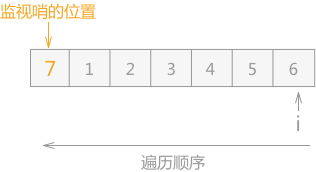
Figure 1 monitoring post in sequence table
At one end of the sequence table, the keyword used by the user for search is added, which is called "monitoring whistle".
The position of the monitoring post in Figure 1 can also be placed after the data element 6 (in this case, the whole search order should be changed from reverse search to sequential search).
After the monitoring whistle is placed, the sequence table is traversed successively from the end without the monitoring whistle. If there is data required by the user in the lookup table, the program outputs the position; On the contrary, the program will run to the monitoring post. At this time, the matching is successful and the program stops running, but the result is that the search fails.
Performance analysis of sequential lookup
The performance analysis of lookup operation mainly considers its time complexity, and most of the time in the whole lookup process is actually spent comparing keywords with the data in the lookup table.
Therefore, the basis for measuring the quality of the search algorithm is: when the search is successful, the average value of the searched keywords and the number of data elements in the search table compared is called the Average Search Length (ASL).
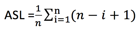
For example, for a lookup table with n data elements, the calculation formula of the average lookup length of successful lookup is:

Pi is the probability of finding the ith data element, and the sum of the probabilities of finding all elements is 1; Ci indicates the number of times the comparison has been made before finding the ith data element. If there are n data elements in the table, the first element needs to be compared n times; The last element needs to be compared once, so there is Ci = n – i + 1.
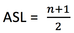
In general, the probability of finding each data element in the table is unknown. Assuming that in the lookup table containing n data elements, the probability of each data being searched is the same, then:
After conversion, the following is obtained:
If the probability that each data element in the lookup table may be searched is known in advance, the data elements in the lookup table should be adjusted appropriately according to the size of its search probability: the greater the search probability, the closer it is to the search starting point i; On the contrary, the farther away. This can appropriately reduce the number of comparisons in the search operation.
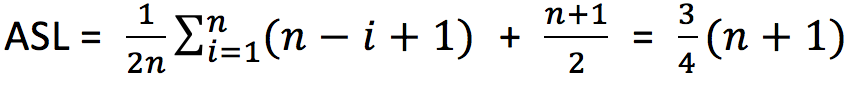
The average search length of the upper edge is obtained on the premise that the search algorithm is successful every time. For the search algorithm, the probability of success and failure is the same. Therefore, the average search length of the search algorithm should be the average search length when the search is successful plus the average search length when the search fails.
For a table containing N data, the number of comparisons is n+1 for each lookup failure. Therefore, the calculation formula of the average search length of the search algorithm is:
summary
This section mainly introduces the representation of sequential storage of static lookup table and the implementation of lookup algorithm, in which the monitoring whistle is used to improve the traversal algorithm of ordinary sequential table, which can effectively improve the operation efficiency of the algorithm in the case of large amount of data.
**
3. Detailed explanation of binary search (half search) algorithm (implemented in C language)
**
Half search, also known as binary search, is more efficient than sequential search in some cases. However, the premise of using this algorithm is that the data in the static lookup table must be orderly.
For example, before the {5,21,13,19,37,75,56,64,88, 80,92} lookup table uses the half search algorithm to find data, you need to sort the data in the table according to the queried Keywords: {5,13,19,21,37,56,64,75,80,88,92}.
Sorting the lookup table according to the queried keyword before half search means that if the data elements stored in the lookup table contain multiple keywords, which keyword is used for half search, you need to sort all data with this keyword in advance.
Half search algorithm
For the static lookup table {5,13,19,21,37,56,64,75,80,88,92}, the process of using the half search algorithm to find the keyword 21 is as follows:
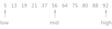
Figure 1 process of half search (a)
As shown in Figure 1 above, the pointers low and high point to the first keyword and the last keyword of the lookup table respectively, and the pointer mid points to the keyword in the middle of the low and high pointers. In the process of searching, the keyword pointed to by mid is compared every time. Because the data in the whole table is orderly, you can know the approximate position of the keyword to be searched after comparison.
For example, when looking up the keyword 21, first compare it with 56. Since 21 < 56 and the lookup table is sorted in ascending order, it can be determined that if there is the keyword 21 in the static lookup table, it must exist in the middle of the area pointed to by low and mid.
Therefore, when traversing again, you need to update the positions of the high pointer and the mid pointer, make the high pointer move to a position to the left of the mid pointer, and make the mid point to the middle of the low pointer and the high pointer again. As shown in Figure 2:
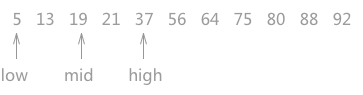
Figure 2 process of half search (b)
Similarly, comparing 21 with 19 pointed by mid pointer, 19 < 21, so it can be determined that 21, if it exists, must be in the area pointed by mid and high. Therefore, make the low point to a position on the right side of the mid, and update the position of the mid at the same time.
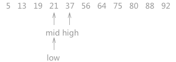
Figure 3 process of half search (3)
When making a judgment for the third time, it is found that mid is keyword 21, and the search ends.
Note: in the process of searching, if the middle position of the low pointer and the high pointer is between the two keywords during calculation, that is, the position of the mid is not an integer, it needs to be rounded uniformly.
Implementation code of half search:
#include <stdio.h>
#include <stdlib.h>
#define keyType int
typedef struct {
    keyType key;//Find the value of each data element in the table
    //If necessary, you can add additional attributes
}ElemType;
typedef struct{
    ElemType *elem;//An array that holds data elements in a lookup table
    int length;//Record the total amount of data in the lookup table
}SSTable;
//Create lookup table
void Create(SSTable **st,int length){
    (*st)=(SSTable*)malloc(sizeof(SSTable));
    (*st)->length=length;
    (*st)->elem = (ElemType*)malloc((length+1)*sizeof(ElemType));
    printf("Data elements in the input table:\n");
    //According to the total length of data elements in the lookup table, data is stored from the space with array subscript 1
    for (int i=1; i<=length; i++) {
        scanf("%d",&((*st)->elem[i].key));
    }
}
//Half search algorithm
int Search_Bin(SSTable *ST,keyType key){
    int low=1;//The initial state low pointer points to the first keyword
    int high=ST->length;//high points to the last keyword
    int mid;
    while (low<=high) {
        mid=(low+high)/2;//int itself is an integer, so mid is a rounded integer every time
        if (ST->elem[mid].key==key)//If the mid points to the same location as the one to be searched, the location pointed to by the mid is returned
        {
            return mid;
        }else if(ST->elem[mid].key>key)//If the keyword pointed to by mid is large, the position of the high pointer is updated
        {
            high=mid-1;
        }
        //Otherwise, the position of the low pointer is updated
        else{
            low=mid+1;
        }
    }
    return 0;
}
int main(int argc, const char * argv[]) {
    SSTable *st;
    Create(&st, 11);
    getchar();
    printf("Please enter a keyword to find data:\n");
    int key;
    scanf("%d",&key);
    int location=Search_Bin(st, key);
    //If the return value is 0, it proves that the key value is not found in the lookup table,
    if (location==0) {
        printf("The element does not exist in the lookup table");
    }else{
        printf("The position of the data in the lookup table is:%d",location);
    }
    return 0;
}
Taking the lookup table in Figure 1 as an example, the operation result is:
Data elements in the input table:
5 13 19 21 37 56 64 75 80 88 92
Please enter a keyword to find data:
21
The position of the data in the lookup table is: 4
Performance analysis of half search
The running process of half search can be described by binary tree, which is usually called "decision tree". For example, in the static lookup table in Figure 1, the corresponding decision tree is shown in Figure 4:
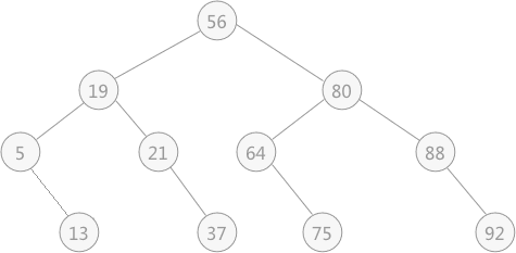
Fig. 4 corresponding decision tree of half search
Note that the leaf node in this figure looks like the right child node of the parent node, but it is not. The leaf node here can be treated as either a right child node or a left child node.
It can be seen in the decision tree that if you want to find the position of 21 in the lookup table, you only need to compare it three times, and compare it with 56, 19 and 21 in turn, and the number of comparisons is exactly the level in the decision tree where the keyword is located (the keyword 21 is at the third level in the decision tree).
For a decision tree with n nodes (the lookup table contains n keywords), the number of layers is at most: log2n + 1 (if the result is not an integer, round it, for example:
log211 +1 = 3 + 1 = 4 ).
Meanwhile, when the search probability of each keyword in the lookup table is the same, the average search length of half search is ASL = log2(n+1) – 1.
summary
By comparing the average search length of half search, compared with the sequential search described earlier, it is obvious that the efficiency of half search is higher. However, the half search algorithm is only applicable to ordered tables, and is limited to lookup tables, which are represented by sequential storage structure.
When the lookup table is represented by a chain storage structure, the half lookup algorithm can not effectively carry out the comparison operation (the implementation of sorting and lookup operations are extremely cumbersome).
**
4. Binary sort tree (binary search tree) and C language implementation
**
The previous sections introduce the knowledge about static lookup tables. Starting from this section, we introduce another kind of lookup table - dynamic lookup table.
When a dynamic lookup table is searched, it can be deleted if the search is successful; If the search fails, that is, the keyword does not exist in the table, you can insert the keyword into the table.
There are many ways to represent dynamic lookup tables. This section introduces an implementation method of using tree structure to represent dynamic lookup tables - binary sort tree (also known as "binary lookup tree").
What is a binary sort tree?
Binary sort tree is either an empty binary tree or has the following characteristics:
In a binary sort tree, if the root node has a left subtree, the values of all nodes on the left subtree are less than those of the root node;
In a binary sort tree, if the root node has a right subtree, the values of all nodes on the right subtree are larger than the values of the root node;
The left and right subtrees of a binary sort tree are also required to be binary sort trees;
For example, figure 1 is a binary sort tree:
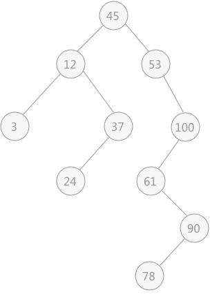
Figure 1 binary sort tree
Use binary sort tree to find keywords
When searching for a keyword in a binary sort tree, the search process is similar to a suboptimal binary tree. On the premise that the binary sort tree is not an empty tree, first compare the searched value with the root node of the tree
3 different results:
If equal, the search is successful;
If the comparison result is that the keyword value of the root node is large, it indicates that the keyword may exist in its left subtree;
If the comparison result is that the keyword value of the root node is small, it indicates that the keyword may exist in its right subtree;
The implementation function is: (using recursive method)
BiTree SearchBST(BiTree T,KeyType key){
    //If T is NULL during recursion, the search result will be NULL; Or if the search is successful, a pointer to the keyword is returned
    if (!T || key==T->data) {
        return T;
    }else if(key<T->data){
        //Recursively traverses its left child
        return SearchBST(T->lchild, key);
    }else{
        //Recursively traverses its right child
        return SearchBST(T->rchild, key);
    }
}
Insert keyword in binary sort tree
Binary sort tree itself is a representation of dynamic lookup table. Sometimes, elements in the table will be inserted or deleted during the lookup process. When a data element needs to be inserted because the lookup fails, the insertion position of the data element must be located in the leaf node of binary sort tree, and must be the left child or right child of the last node accessed when the lookup fails.
For example, in the binary sort tree in Figure 1, you can find keyword 1. When you find the leaf node of keyword 3, it is judged that there is no keyword in the table. At this time, the insertion position of keyword 1 is the left child of keyword 3.
Therefore, the binary sort tree indicates that the dynamic lookup table can be inserted only by slightly changing the above code. The specific implementation code is as follows:
BOOL SearchBST(BiTree T,KeyType key,BiTree f,BiTree *p){
    //If the T pointer is empty, the search fails. Make the p pointer point to the last leaf node in the search process and return the information of search failure
    if (!T){
        *p=f;
        return false;
    }
    //If equal, make the p pointer point to the keyword and return the search success information
    else if(key==T->data){
        *p=T;
        return true;
    }
    //If the key value is smaller than the value of the T root node, find its left subtree; On the contrary, find its right subtree
    else if(key<T->data){
        return SearchBST(T->lchild,key,T,p);
    }else{
        return SearchBST(T->rchild,key,T,p);
    }
}
//Insert function
BOOL InsertBST(BiTree T,ElemType e){
    BiTree p=NULL;
    //If the search is unsuccessful, you need to insert
    if (!SearchBST(T, e,NULL,&p)) {
        //Initialize insert node
        BiTree s=(BiTree)malloc(sizeof(BiTree));
        s->data=e;
        s->lchild=s->rchild=NULL;
        //If p is NULL, the binary sort tree is empty, and the inserted node is the root node of the whole tree
        if (!p) {
            T=s;
        }
        //If P is not NULL, then p points to the last leaf node that failed to find. Just compare the values of P and e to determine whether s is the left child or the right child of P
        else if(e<p->data){
            p->lchild=s;
        }else{
            p->rchild=s;
        }
        return true;
    }
    //If the search is successful, no insertion operation is required, and the insertion fails
    return false;
}
By using the binary sort tree to search and insert the dynamic lookup table, and when traversing the binary sort tree in middle order, we can get an ordered sequence of all keywords.
For example, assuming that the original binary sort tree is an empty tree, when searching and inserting the dynamic lookup table {3, 5, 7, 2, 1}, you can build a binary sort tree containing all the keywords in the table, as shown in Figure 2:
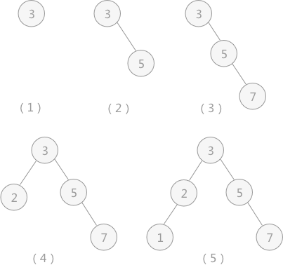
Figure 2 insertion process of binary sort tree
Through continuous search and insertion operations, the final binary sort tree is shown in Figure 2 (5). When the middle order traversal algorithm is used to traverse the binary sort tree, the sequence is: 1 2 3 5 7, which is an ordered sequence.
An unordered sequence can be transformed into an ordered sequence by constructing a binary sorting tree.
Delete keyword from binary sort tree
In the process of searching, if a data element is deleted from the dynamic lookup table represented by binary sort tree, the tree needs to be binary sort tree while successfully deleting the node.
Assuming that the node to be deleted is node p, for a binary sort tree, different operations need to be performed according to the different positions of node p. there are three possibilities:
1. Node p is a leaf node. In this case, you only need to delete the node and modify the pointer of its parent node;
2. Node p has only left subtree or right subtree. If p is the left child of its parent node, the left subtree or right subtree of node p is directly taken as the left subtree of its parent node; On the contrary, if p is the right child of its parent node, the left subtree or right subtree of p node is directly taken as the right subtree of its parent node;
3. There are both left and right subtrees of node p. at this time, there are two processing methods:
1) Let the left subtree of node p be the left subtree of its parent node; The right subtree of node P is the right subtree of its own direct precursor node, as shown in Figure 3;
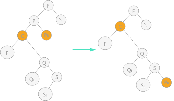
Figure 3 deleting nodes in binary sort tree (1)
2) Replace node p with the direct precursor (or direct successor) of node p, and delete its direct precursor (or direct successor) in the binary sort tree. As shown in Figure 4, the direct precursor is used instead of node p:
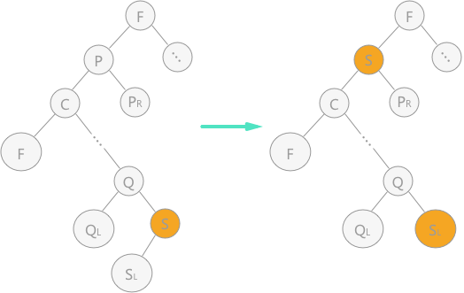
Figure 4 deleting nodes in binary sort tree (2)
In Fig. 4, in the middle order traversal of the left graph, the direct precursor node of node p is node s, so node s is directly used to cover node p. since node s has left children, it is directly changed into the right children of parent nodes according to rule 2.
Specific implementation code: (runnable)
#include<stdio.h>
#include<stdlib.h>
#define TRUE 1
#define FALSE 0
#define ElemType int
#define  KeyType int
/* Node structure definition of binary sort tree */
typedef struct BiTNode
{
    int data;
    struct BiTNode *lchild, *rchild;
} BiTNode, *BiTree;
//Binary sort tree search algorithm
int SearchBST(BiTree T, KeyType key, BiTree f, BiTree *p) {
    //If the T pointer is empty, the search fails. Make the p pointer point to the last leaf node in the search process and return the information of search failure
    if (!T) {
        *p = f;
        return FALSE;
    }
    //If equal, make the p pointer point to the keyword and return the search success information
    else if (key == T->data) {
        *p = T;
        return TRUE;
    }
    //If the key value is smaller than the value of the T root node, find its left subtree; On the contrary, find its right subtree
    else if (key < T->data) {
        return SearchBST(T->lchild, key, T, p);
    }
    else {
        return SearchBST(T->rchild, key, T, p);
    }
}
int InsertBST(BiTree *T, ElemType e) {
    BiTree p = NULL;
    //If the search is unsuccessful, you need to insert
    if (!SearchBST((*T), e, NULL, &p)) {
        //Initialize insert node
        BiTree s = (BiTree)malloc(sizeof(BiTNode));
        s->data = e;
        s->lchild = s->rchild = NULL;
        //If p is NULL, the binary sort tree is empty, and the inserted node is the root node of the whole tree
        if (!p) {
            *T = s;
        }
        //If P is not NULL, then p points to the last leaf node that failed to find. Just compare the values of P and e to determine whether s is the left child or the right child of P
        else if (e < p->data) {
            p->lchild = s;
        }
        else {
            p->rchild = s;
        }
        return TRUE;
    }
    //If the search is successful, no insertion operation is required, and the insertion fails
    return FALSE;
}
//Delete function
int Delete(BiTree *p)
{
    BiTree q, s;
    //In case 1, node p itself is a leaf node and can be deleted directly
    if (!(*p)->lchild && !(*p)->rchild) {
        *p = NULL;
    }
    else if (!(*p)->lchild) { //If the left subtree is empty, just use the root node of the right subtree of node p to replace node p;
        q = *p;
        *p = (*p)->rchild;
        free(q);
    }
    else if (!(*p)->rchild) {//If the right subtree is empty, just use the root node of the left subtree of node p to replace node p;
        q = *p;
        *p = (*p)->lchild;//Here, instead of the pointer * p pointing to the left subtree, the address of the node stored in the left subtree is assigned to the pointer variable p
        free(q);
    }
    else {//The left and right subtrees are not empty. The second method is adopted
        q = *p;
        s = (*p)->lchild;
        //Traverse to find the direct precursor of node p
        while (s->rchild)
        {
            q = s;
            s = s->rchild;
        }
        //Directly change the value of node p
        (*p)->data = s->data;
        //Whether the left subtree s of node p has a right subtree is discussed in two cases
        if (q != *p) {
            q->rchild = s->lchild;//If yes, while deleting the direct precursor node, change the left child node of the precursor to the child node q pointing to the node
        }
        else {
            q->lchild = s->lchild;//Otherwise, move the left subtree up directly
        }
        free(s);
    }
    return TRUE;
}
int DeleteBST(BiTree *T, int key)
{
    if (!(*T)) {//There is no data element with keyword equal to key
        return FALSE;
    }
    else
    {
        if (key == (*T)->data) {
            Delete(T);
            return TRUE;
        }
        else if (key < (*T)->data) {
            //Use recursion
            return DeleteBST(&(*T)->lchild, key);
        }
        else {
            return DeleteBST(&(*T)->rchild, key);
        }
    }
}
void order(BiTree t)//Medium sequence output
{
    if (t == NULL) {
        return;
    }
    order(t->lchild);
    printf("%d ", t->data);
    order(t->rchild);
}
int main()
{
    int i;
    int a[5] = { 3,4,2,5,9 };
    BiTree T = NULL;
    for (i = 0; i < 5; i++) {
        InsertBST(&T, a[i]);
    }
    printf("Traversing binary sort tree in middle order:\n");
    order(T);
    printf("\n");
    printf("After deleting 3, traverse the binary sort tree in middle order:\n");
    DeleteBST(&T, 3);
    order(T);
}
Operation results:
Traversing binary sort tree in middle order:
2 3 4 5 9
After deleting 3, traverse the binary sort tree in middle order:
2 4 5 9
summary
The time complexity of using binary sort tree to do lookup operation in lookup table is related to the structure of the established binary tree itself. Even if the data elements in the lookup table are exactly the same, the binary sort tree constructed is very different with different sort order.
For example, the binary sort tree constructed by lookup table {45, 24, 53, 12, 37, 93} and table {12, 24, 37, 45, 53, 93} is shown in the following figure:
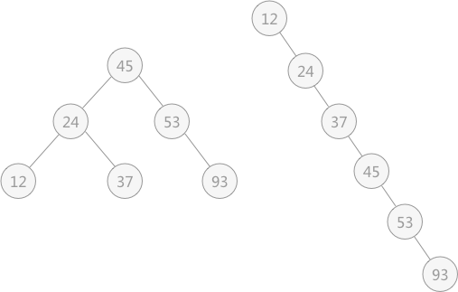
Fig. 5 binary sort trees with different structures
**
5. Balanced binary tree (AVL tree) and C language implementation
**
The previous section describes how to use binary sort tree to realize dynamic lookup table. This section introduces another implementation method - balanced binary tree.
Balanced binary tree, also known as AVL tree. In fact, it is a binary tree that follows the following two characteristics:
The depth difference between the left subtree and the right subtree in each subtree shall not exceed 1;
Each subtree in a binary tree is required to be a balanced binary tree;
In fact, on the basis of binary tree, if each subtree in the tree satisfies that the depth difference between its left subtree and right subtree is no more than 1, then the binary tree is a balanced binary tree.
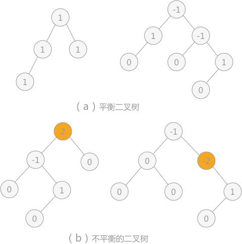
Figure 1 balanced and unbalanced binary tree and node balance factor
Balance factor: each node has its own balance factor, which represents the difference between the depth of its left subtree and that of its right subtree. The values of the balance factor of each node in the balanced binary tree can only be 0, 1 and - 1.
As shown in Figure 1, in the two binary trees in (a), since the absolute value of the number of balance factors of each node does not exceed 1, the two binary trees in (a) are balanced binary trees; The absolute value of the number of balance factors of nodes in the two binary trees of (b) exceeds 1, so they are not balanced binary trees.
Binary sort tree into balanced binary tree
In order to eliminate the influence of different data arrangement modes in the dynamic lookup table on the performance of the algorithm, it is necessary to consider transforming the binary sort tree into a balanced binary tree without damaging the structure of the binary sort tree itself.
For example, when using the algorithm in the previous section to build a binary sort tree for the lookup table {13, 24, 37, 90, 53}, when inserting 13 and 24, the binary sort tree is still a balanced binary tree:
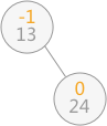
Figure 2 balanced binary tree
When inserting 37, the structure of the generated binary sort tree is damaged, as shown in Figure 3 (a). At this time, only the "rotation" operation is required for the binary sort tree (as shown in Figure 3 (b)), that is, the whole tree takes node 24 as the root node, the structure of the binary sort tree is not damaged, and the tree is transformed into a balanced binary tree:
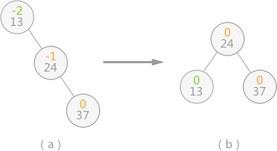
Fig. 3 process of binary sort tree changing into balanced binary tree
When the balance of the binary sort tree is broken, it is like the phenomenon that one end is heavy and the other end is light at both ends of the shoulder pole, as shown in Figure 3 (a). At this time, it can be restored to balance only by changing the support point of the shoulder pole (the root of the tree). In fact, in Figure 3 (b), the binary tree of (a) is rotated to the left and counterclockwise.
After inserting 90 and 53, the binary sort tree is shown in Fig. 4 (a), resulting in the absolute value of the balance factor of nodes 24 and 37 in the binary tree is greater than 1, and the balance of the whole tree is broken. At this point, you need to do two steps:
As shown in Fig. 4 (b), rotate nodes 53 and 90 clockwise to the right, so that the subtree with 90 as the root node changes to node 53 as the root node;
As shown in Fig. 4 (c), rotate the subtree with node 37 as the root node to the left counterclockwise to change the subtree with 37 as the root node to node 53 as the root node;
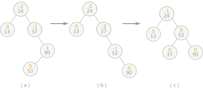
Figure 4 transformation of binary sort tree into balanced binary tree
After the above operations, the unbalanced binary sort tree is transformed into a balanced binary tree.
When the balance of the balanced binary tree is damaged due to the new data elements, it needs to make appropriate adjustments according to the actual situation. It is assumed that the "imbalance factor" closest to the insertion node is a. Then the regulation can be summarized into the following four cases:
Unidirectional right rotation balance processing: if the left subtree of node a is inserted into the left subtree of the root node, resulting in the balance factor of node a increasing from 1 to 2, resulting in the loss of balance of the subtree with a as the root node, only one clockwise rotation to the right is required, as shown in the figure below:
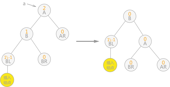
Fig. 5 unidirectional right rotation
One way left rotation balance processing: if the balance factor of node a changes from - 1 to - 2 because the right subtree of node a is inserted into the right subtree of the root node, the subtree with a as the root node needs to rotate counterclockwise to the left, as shown in the following figure:
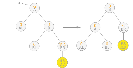
Fig. 6 unidirectional left rotation
Bidirectional rotation (left first and then right) balancing: if the left subtree of node a is inserted into the right subtree of the root node, resulting in the balance factor of node a increasing from 1 to 2, resulting in the loss of balance of the subtree with a as the root node, two rotation operations are required, as shown in the figure below:
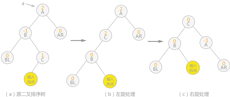
Fig. 7 bidirectional rotation (first left and then right)
Note: the inserted node in Figure 7 can also be the right child of node C, then the position of the inserted node in (b) is still the right child of node C, and the position of the inserted node in (c) is the left child of node A.
Bidirectional rotation (right before left) balancing: if the right subtree of node a is inserted into the left subtree of the root node, resulting in the balance factor of node a changing from - 1 to - 2, resulting in the loss of balance of the subtree with a as the root node, two rotations (right before left) are required, as shown in the following figure:
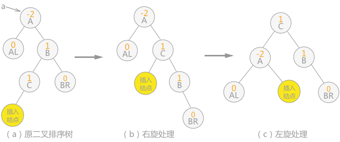
Fig. 8 bidirectional rotation (first right then left)
Note: the inserted node in Figure 8 can also be the right child of node C, then the position of the inserted node in (b) is changed to the left child of node B, and the position of the inserted node in (c) is the left child of node B.
When building a balanced binary tree for the lookup table {13, 24, 37, 90, 53}, because it conforms to the law of Article 4, it is processed from right rotation to left rotation, and finally transformed from an unbalanced binary sort tree to a balanced binary tree.
Code implementation of constructing balanced binary tree
#include <stdio.h>
#include <stdlib.h>
//Define the number of balance factors respectively
#define LH +1
#define EH  0
#define RH -1
typedef int ElemType;
typedef enum {false,true} bool;
//Define binary sort tree
typedef struct BSTNode{
    ElemType data;
    int bf;//balance flag
    struct BSTNode *lchild,*rchild;
}*BSTree,BSTNode;
//Right rotate the binary tree with p as the root node, and make the p pointer point to the new tree root node
void R_Rotate(BSTree* p)
{
    //It is understood with the help of Figure 5 in the article, where node A is the root node pointed to by the p pointer
    BSTree lc = (*p)->lchild;
    (*p)->lchild = lc->rchild;
    lc->rchild = *p;
    *p = lc;
}
To p Do left-handed processing for the binary tree of the root node, so that p The pointer points to the new tree root node
void L_Rotate(BSTree* p)
{
    //It is understood with the help of Figure 6 in the article, where node A is the root node pointed to by the p pointer
    BSTree rc = (*p)->rchild;
    (*p)->rchild = rc->lchild;
    rc->lchild = *p;
    *p = rc;
}
//Balance the left subtree of the binary tree with the node pointed to by pointer T as the root node, so that pointer T points to the new root node
void LeftBalance(BSTree* T)
{
    BSTree lc,rd;
    lc = (*T)->lchild;
    //Check the reasons for the loss of balance of the subtree with the left subtree of T as the root node. If bf value is 1, it indicates that it is added to the left subtree with the left subtree as the root node and needs to be right rotated; On the contrary, if bf value is - 1, it indicates that adding to the right subtree with the left subtree as the root node requires two-way left rotation first and then right rotation
    switch (lc->bf)
    {
        case LH:
            (*T)->bf = lc->bf = EH;
            R_Rotate(T);
            break;
        case RH:
            rd = lc->rchild;
            switch(rd->bf)
        {
            case LH:
                (*T)->bf = RH;
                lc->bf = EH;
                break;
            case EH:
                (*T)->bf = lc->bf = EH;
                break;
            case RH:
                (*T)->bf = EH;
                lc->bf = LH;
                break;
        }
            rd->bf = EH;
            L_Rotate(&(*T)->lchild);
            R_Rotate(T);
            break;
    }
}
//The balance processing of the right subtree is completely similar to that of the left subtree
void RightBalance(BSTree* T)
{
    BSTree lc,rd;
    lc= (*T)->rchild;
    switch (lc->bf)
    {
        case RH:
            (*T)->bf = lc->bf = EH;
            L_Rotate(T);
            break;
        case LH:
            rd = lc->lchild;
            switch(rd->bf)
        {
            case LH:
                (*T)->bf = EH;
                lc->bf = RH;
                break;
            case EH:
                (*T)->bf = lc->bf = EH;
                break;
            case RH:
                (*T)->bf = EH;
                lc->bf = LH;
                break;
        }
            rd->bf = EH;
            R_Rotate(&(*T)->rchild);
            L_Rotate(T);
            break;
    }
}
int InsertAVL(BSTree* T,ElemType e,bool* taller)
{
    //If it is an empty tree, add e as the root node directly
    if ((*T)==NULL)
    {
        (*T)=(BSTree)malloc(sizeof(BSTNode));
        (*T)->bf = EH;
        (*T)->data = e;
        (*T)->lchild = NULL;
        (*T)->rchild = NULL;
        *taller=true;
    }
    //If e already exists in the binary sort tree, no processing will be done
    else if (e == (*T)->data)
    {
        *taller = false;
        return 0;
    }
    //If e is smaller than the data field of node T, it is inserted into the left subtree of T
    else if (e < (*T)->data)
    {
        //If the insertion process does not affect the balance of the tree itself, it ends directly
        if(!InsertAVL(&(*T)->lchild,e,taller))
            return 0;
        //Determine whether the insertion process will result in the depth of the whole tree + 1
        if(*taller)
        {
            //Judge the balance factor of the root node T. because the balance is lost in the process of adding new nodes to its left subtree, when the balance factor of the T node itself is 1, it is necessary to balance the left subtree, otherwise the number of balance factors of each node in the tree will be updated
            switch ((*T)->bf)
            {
                case LH:
                    LeftBalance(T);
                    *taller = false;
                    break;
                case  EH:
                    (*T)->bf = LH;
                    *taller = true;
                    break;
                case RH:
                    (*T)->bf = EH;
                    *taller = false;
                    break;
            }
        }
    }
    //Similarly, when E > T - > data, you need to insert it into the right subtree of the tree with t as the root node. You also need to do the same operation as above
    else
    {
        if(!InsertAVL(&(*T)->rchild,e,taller))
            return 0;
        if (*taller)
        {
            switch ((*T)->bf)
            {
                case LH:
                    (*T)->bf = EH;
                    *taller = false;
                    break;
                case EH:
                    (*T)->bf = RH;
                    *taller = true;
                    break;
                case  RH:
                    RightBalance(T);
                    *taller = false;
                    break;
            }
        }
    }
    return 1;
}
//Judge whether the existing balanced binary tree already has a node with data field e
bool FindNode(BSTree root,ElemType e,BSTree* pos)
{
    BSTree pt = root;
    (*pos) = NULL;
    while(pt)
    {
        if (pt->data == e)
        {
            //Find the node, and pos points to the node and returns true
            (*pos) = pt;
            return true;
        }
        else if (pt->data>e)
        {
            pt = pt->lchild;
        }
        else
            pt = pt->rchild;
    }
    return false;
}
//Middle order ergodic balanced binary tree
void InorderTra(BSTree root)
{
    if(root->lchild)
        InorderTra(root->lchild);

    printf("%d ",root->data);

    if(root->rchild)
        InorderTra(root->rchild);
}
int main()
{
    int i,nArr[] = {1,23,45,34,98,9,4,35,23};
    BSTree root=NULL,pos;
    bool taller;
    //Building a balanced binary tree with nArr lookup table (the process of constantly inserting data)
    for (i=0;i<9;i++)
    {
        InsertAVL(&root,nArr[i],&taller);
    }
    //Middle order traversal output
    InorderTra(root);
    //Judge whether the balanced binary tree contains data with data field 103
    if(FindNode(root,103,&pos))
        printf("\n%d\n",pos->data);
    else
        printf("\nNot find this Node\n");
    return 0;
}
Operation results
1 4 9 23 34 35 45 98
Not find this Node
summary
The time complexity of finding using balanced binary tree is O(logn). When learning the contents of this section, it is easier to understand the illustrations close to this section.
**
6. Detailed explanation of hash table (hash table) (including hash table conflict handling methods)
**
The static lookup table and some lookup methods in the dynamic lookup table are introduced earlier. The lookup process can not avoid comparing with the data in the lookup table. The efficiency of the lookup algorithm largely depends on the lookup times of the data in the same table.
The hash table described in this section can directly find the storage location of data through keywords without any comparison. Its search efficiency is higher than the search algorithm described above.
Construction of hash table
I learned the relevant knowledge of function in the mathematics textbook of junior middle school. Given an x, through a mathematical formula, I only need to bring the value of x into the formula to find a new value y.
The establishment of hash table is similar to the function. Replace x in the function with the keyword used to find the record, and then bring the value of the keyword into a carefully designed formula to find a value, which is used to represent the hash address stored in the record. Namely:
Hash address of data = f (value of keyword)
The hash address only represents the storage location in the lookup table, not the actual physical storage location. f () is a function that can quickly find the hash address of the data corresponding to the keyword, which is called "hash function".
For example, here is a phone book (look-up table), which contains the contact information of 4 people:
Zhang San 13912345678
Li Si 15823457890
Wang Wu 13409872338
Zhao Liu 13805834722
If you want to find Li Si's phone number, for the general search method, the first thing you think of is to traverse from scratch and compare them one by one. If you build the phone book into a hash table, you can directly find the location of the phone number in the table through the name "Li Si".
When building a hash table, the most important thing is the design of hash function. For example, the hash function in the design phone book case is: the ASCII value of the first letter of each first name is the storage location of the corresponding phone number. At this time, it will be found that the first letter of the surname of Zhang San and Zhao Liu is Z, and the storage location of the final phone number is the same. This phenomenon is called conflict. When designing hash functions, we should try to avoid conflicts.
For hash tables, conflicts can only be as few as possible and cannot be completely avoided.
Construction of hash function
There are six common construction methods of hash function: direct addressing method, digital analysis method, square middle method, folding method, division and residue method and random number method.
Direct addressing method: its hash function is a primary function, that is, the following two forms:
H (key) = key or H (key) = a * key + b
Where H (key) represents the hash address corresponding to the key, and a and b are constants.
For example, there is a demographic table from 1 to 100 years old, as shown in Table 1:
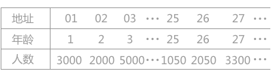
Table 1 demographic table
Suppose its hash function is the first form, and the value of its keyword represents the final storage location. If it is necessary to find the population aged 25, bring the age 25 into the hash function and directly obtain the corresponding hash address of 25 (the obtained hash address indicates that the position of the record is in the 25th bit of the lookup table).
Digital analysis method: if the keyword consists of multiple characters or numbers, you can consider extracting 2 or more of them as the hash address corresponding to the keyword, and try to select the bits with more changes in the extraction method to avoid conflicts.
For example, some keywords are listed in Table 2, and each keyword is composed of 8 decimal digits:
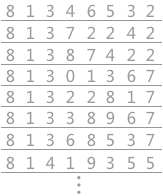
Table 2
By analyzing the composition of the keyword, it is obvious that the first and second bits of the keyword are fixed, and the third bit is either the number 3 or 4. The last bit can only take 2, 7 and 5, and only the middle four bits have approximate random values. Therefore, in order to avoid conflict, 2 bits can be arbitrarily selected from the four bits as its hash address.
The square middle method is to square the keyword and take the middle bits as the hash address. This method is also a common method to construct hash function.
For example, if the keyword sequence is {421423436}, and the result after squaring each keyword is {1772411789291096}, the middle two bits {72, 89, 00} can be taken as its hash address.
The folding method is to divide the keyword into several parts with the same number of bits (the number of bits of the last part can be different), and then take the superposition and (round off the carry) of these parts as the hash address. This method is suitable for the situation with more keyword digits.
For example, in the library, books are numbered with a 10 digit decimal number as the keyword. If a hash table is established for its lookup table, the folding method can be used.
If the number of a book is 0-442-20586-4, the division method is shown in Figure 1. There are two ways to fold it: displacement folding and boundary folding:
Shift folding is to align each small part after segmentation according to its lowest position, and then add it, as shown in Fig. 1 (a);
The boundary folding is to fold back and forth along the division line from one end to the other end, as shown in Fig. 1 (b).
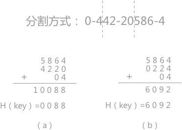
Figure 1 displacement folding and boundary folding
Divide and leave remainder method: if the maximum length m of the whole hash table is known, take a number P not greater than m, and then perform remainder operation on the keyword key, that is, H (key) = key% p.
In this method, the value of p is very important. It is known from experience that p can be a prime number not greater than m or a composite number without a prime factor less than 20.
Random number method: it takes a random function value of the keyword as its hash address, that is, H (key) = random (key). This method is applicable to the case of different keyword lengths.
Note: the random function here is actually a pseudo-random function. The random function is that even if the given key is the same every time, H (key) is different; The pseudo-random function is just the opposite. Each key corresponds to a fixed H (key).
When selecting so many methods to build hash functions, we need to take appropriate methods according to the actual lookup table. The following factors are usually considered:
The length of the keyword. If the length is not equal, the random number method is selected. If the number of key words is large, the folding method or digital analysis method shall be selected; On the contrary, if the number of digits is short, the square median method can be considered;
The size of the hash table. If the size is known, the division and remainder method can be selected;
Distribution of keywords;
Lookup frequency of lookup table;
The time required to calculate the hash function (including the factors of hardware instructions)
Methods of handling conflicts
For the establishment of hash table, we need to select the appropriate hash function, but for unavoidable conflicts, we need to take appropriate measures to deal with them.
The following methods are commonly used to deal with conflicts:
Open addressing method H (key) = (H (key) + d) MOD m (where m is the table length of the hash table and d is an increment). When the obtained hash address conflicts, select one of the following three methods to obtain the value of d, and then continue the calculation until the calculated hash address is not in conflict. The three methods are:
Linear detection method: d=1, 2, 3,..., m-1
Secondary detection method: d=12, - 12, 22, - 22, 32
Pseudo random number detection method: d = pseudo random number
For example, in the hash table with a length of 11, the three data 17, 60 and 29 have been filled in (as shown in Fig. 2 (a)), in which the hash function used is: H (key) = key MOD 11. For the existing fourth data 38, when the hash address obtained by the hash function is 5, which conflicts with 60, the above three methods are used to obtain the insertion position respectively, as shown in Fig. 2 (b):
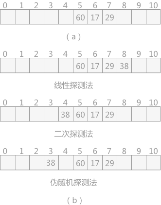
Figure 2 open addressing method
Note: in the linear detection method, in case of conflict, from the position where the conflict occurs, + 1 each time, and detect to the right until there is a free position; In the secondary detection method, from the position where the conflict occurs, detect according to + 12, - 12, + 22,... Until there is a free position; Pseudo random detection, adding a random number each time until the end of detecting an idle position.
double hashing
When the hash address obtained by the hash function conflicts with other keywords, another hash function is used for calculation until the conflict no longer occurs.
Chain address method
The data corresponding to all conflicting keywords are stored in the same linear linked list. For example, a group of keywords are {19,14,23,01,68,20,84,27,55,11,10,79}, and its hash function is: H(key)=key MOD 13. The hash table constructed by using the chain address method is shown in Figure 3:
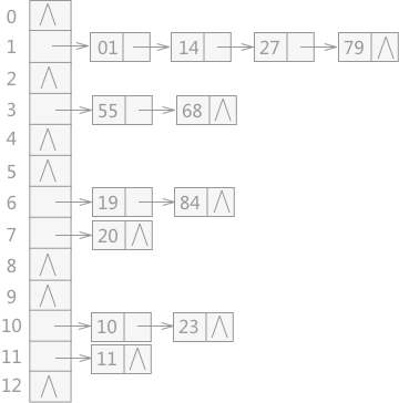
Figure 3 hash table constructed by chain address method
Establish a common overflow area
Create two tables, one for the basic table and the other for the overflow table. The basic table stores data without conflict. When the hash address generated by the hash function conflicts, the data will be filled into the overflow table.
summary
This section mainly introduces the construction of hash table and the methods to deal with conflicts during the construction process. When selecting which method to use, it is necessary to analyze the specific problems according to the actual situation of the lookup table.