Chapter 5 logistic regression algorithm

   based on the linear regression algorithm, the logical regression algorithm constructs the conversion function of the dependent variable y, and divides the number of Y into two or more categories of 0-1, so as to realize the classification fitting and prediction of things.

5.1 from linear regression to classification problem

• Regression method is an algorithm for predicting and modeling continuous random variables.
    forecast house prices, stock trends, commodity sales, etc.
• Classification method is an algorithm for modeling or predicting discrete random variables
    filter spam, financial fraud, predict whether the evaluation is positive or negative, etc.
• The characteristic of regression task is that the labeled data set is continuous random variable
• The classification algorithm is suitable for predicting a discrete category (probability of category)

5.2 classification based on Sigmoid function

   logistic regression is classified based on Sigmoid function. The function form is:

• chart

5.3 find the optimal solution by gradient descent method

   similar to linear regression, the parameter solution of logical regression is also based on the optimization principle of cost function. However, because the output value of logical regression is discontinuous, log likelihood cost function or log likelihood loss function is usually used to establish the equation for parameter solution.

5.3.1 log likelihood function

Probability:
   is the possibility of something happening in a specific environment. It describes the output result of random variables when the parameters are known.
Likelihood:
   is the possible parameter to speculate the result after determining the result, which is used to describe the possible value of the position parameter when the output result of the known random variable.

• The probability function is usually used as p(x)| θ) Representation (to be exact, conditional probability)
     θ Represents the parameter corresponding to the occurrence of the event
     x indicates the result
• The likelihood function is usually used in L( θ| x) Show

Maximum likelihood / maximum likelihood:
   since the likelihood describes the possibility of the event under different conditions when the results are known, the greater the value of the likelihood function, the greater the possibility of the event under the corresponding conditions.
   in the field of machine learning, the reason why we should pay attention to maximum likelihood is that we need to find out the most likely condition to produce this result according to the known events (existing samples / training sets), so that we can infer the probability of unknown events (prediction samples / prediction sets) according to this condition.

5.3.2 parameter solution of gradient descent method

Cost function of logistic regression:

• chart
• The minus sign is added because the maximum likelihood estimation is used to calculate LNL( θ) The gradient descent method is generally used to find the minimum value, so the minus sign can be added to find a minimum parameter by using the gradient descent method θ.

5.4 python implementation of logistic regression

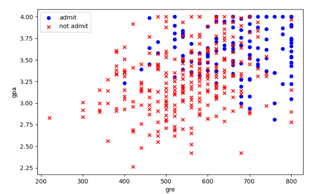
5.4.1 python example of gradient descent method: predicting whether students will be admitted (I)

1. Import data

df = pd.read_csv('D:/PythonProject/machine/data/5_logisitic_admit.csv')
# Insert a column with all 1 in df
df.insert(1,'Ones',1)
# Filter the data with admit of 1 to form a separate data set
positive = df[df['admit'] == 1]
# Filter the data with admit 0 to form a separate data set
negative = df[df['admit'] == 0]

# Create subgraph
fig,ax = plt.subplots(figsize=(8,5))
# Construct positive scatter diagram
ax.scatter(positive['gre'],positive['gpa'],s=30,c='b',marker='o',label='admit')
# Build negative scatter diagram
ax.scatter(negative['gre'],negative['gpa'],s=30,c='r',marker='x',label='not admit')
# Set legend
ax.legend()
# Set x,y axis labels
ax.set_xlabel('gre')
ax.set_ylabel('gpa')
plt.show()

1. Build sigmoid() function and predict() function

# Build sigmoid() function
def sigmoid(z):
    return 1 / (1 + np.exp(-z))

# Building the predict() function
def predict(theta,X):
    # Predict the probability of admit according to sigmoid() function
    prob = sigmoid(X * theta.T)
    # Set the threshold according to the probability of admit. If it is greater than 0.5, it will be recorded as 1, otherwise it will be 0
    return [1 if a >= 0.5 else 0 for a in prob]

1. Build gradient descent() function

"""
    X,y: Input variable
    theta: parameter
    alpha: Learning rate
    m: Number of samples
    numIter: Number of gradient descent iterations
"""

def gradientDescent(X, y, theta, alpha, m, numIter):
    # Matrix transpose
    XTrans = X.transpose()
    # Loop between 1-numIter
    for i in range(0, numIter):
        # Convert theta to matrix
        theta = np.matrix(theta)
        # Convert predicted values to arrays
        pred = np.array(predict(theta, X))
        # See actual value for predicted value
        loss = pred - y
        # Calculated gradient
        gradient = np.dot(XTrans, loss)
        # Calculation of theta parameter, update rule
        theta = theta - alpha * gradient
    return theta

1. Solving parameters by gradient descent method

# Take the last three columns of df as X variables
X = df.iloc[:,1:4]
# Set y variable
y = df['admit']
# Convert X and Y into array form for easy calculation
X = np.array(X.values)
y = np.array(y.values)
# Set the training sample value m and the number of variables n
m,n = np.shape(X)
# initialization
theta = np.ones(n)
# Check whether the row and column numbers of X and y are consistent
print(X.shape,theta.shape,y.shape)
# Number of iterations
numIter = 1000
# Learning rate
alpha = 0.00001
# The constructed gradientDescent() function is used to solve theta
theta = gradientDescent(X,y,theta,alpha,m,numIter)
print('θ={}'.format(theta))

θ=[[ 0.82635 -1.3196 0.7192773]]

1. Predict and calculate accuracy

# Use the predict() function to predict y
pred = predict(theta,X)
# If the forecast is 1, the actual value is 1, the forecast is 0, and the actual value is 0, they are recorded as 1
correct = [1 if((a == 1 and b == 1) or (a ==0 and b == 0))
           else 0 for (a,b) in zip(pred,y)]
# The total correct value is used to calculate the number of prediction pairs
accuracy = (sum(map(int,correct)) % len(correct))
# Print prediction accuracy
print('accurary={:.2f}%'.format(100*accuracy/m))

accurary=67.25%

Data file:
Link: https://pan.baidu.com/s/1TVPNcRKgrDttDOFV8Q2iDA
Extraction code: h4ex