This paper mainly starts with the mathematical principle, and discusses how to make the computer learn the linear regression equation through the known data. Before we go into detail, let's take a look at an example.

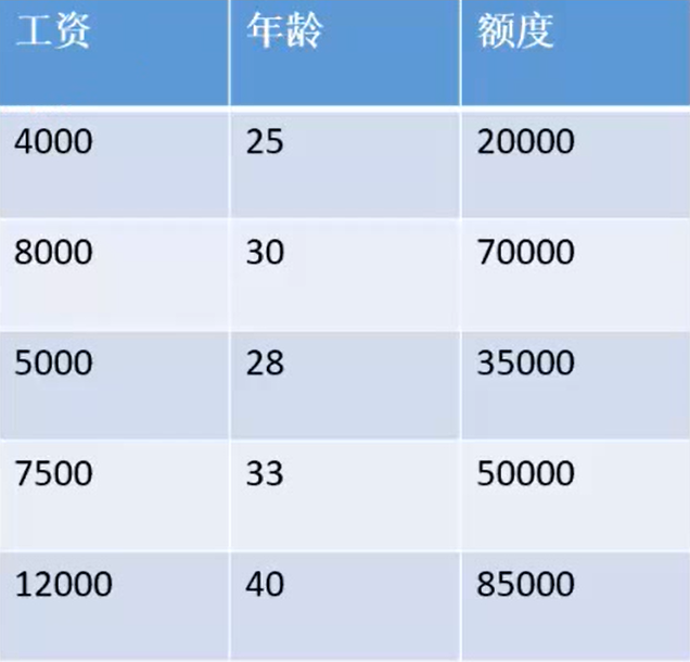
This is a statistical table about the amount of bank loans. It can be seen that in this example, the bank loan amount is related to the borrower's salary and age. In terms of computer language, our prediction function is controlled by two variables. How can we get the linear regression equation of this example? First, from the mathematical aspect, iterate the variables by starting from the functional formula of the prediction function. The following are the detailed steps.

catalogue

1, Mathematical derivation of loss function:

(1) Solving linear regression equation by gradient descent method

(2) Solving linear regression equation by normal equation method

2, Source code display

1, Mathematical derivation of loss function:

The following is the mathematical derivation of loss function, which is not necessary and can be skipped selectively

      

Before the derivation, we can roughly estimate our function model, and the estimation of function model varies from person to person. Different function models will affect the final fitting effect. If the function model is too complex or the dimension is too high, there will be over fitting. This paper will not discuss it. If readers are interested, they can browse the author's blog on regularization, which has a detailed explanation.

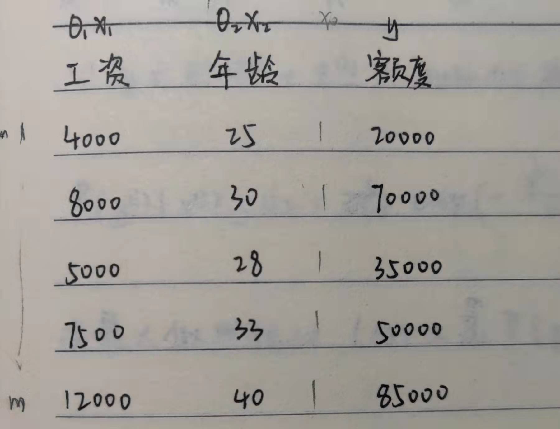
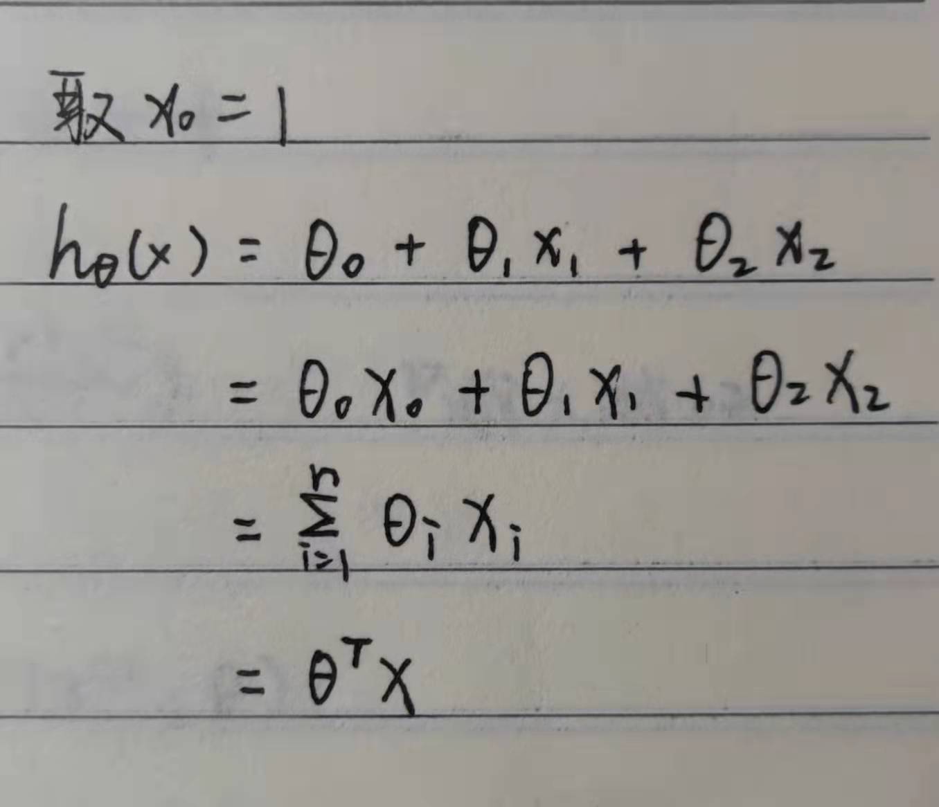
In fact, the introduction of the concept of matrix can greatly facilitate our calculation. If we can't operate the matrix, we can skip this point. Through the concept of matrix, it is obvious that we can get: the transpose of prediction function = theta times matrix x

        

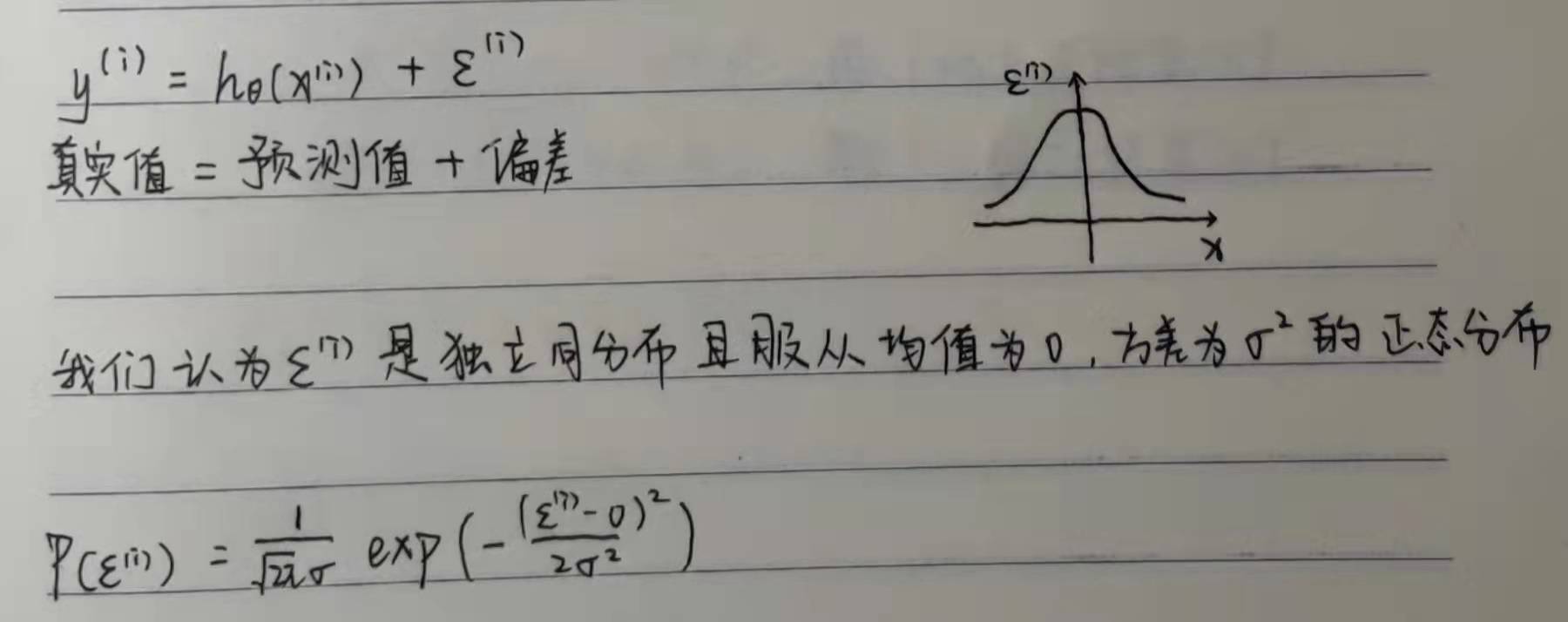
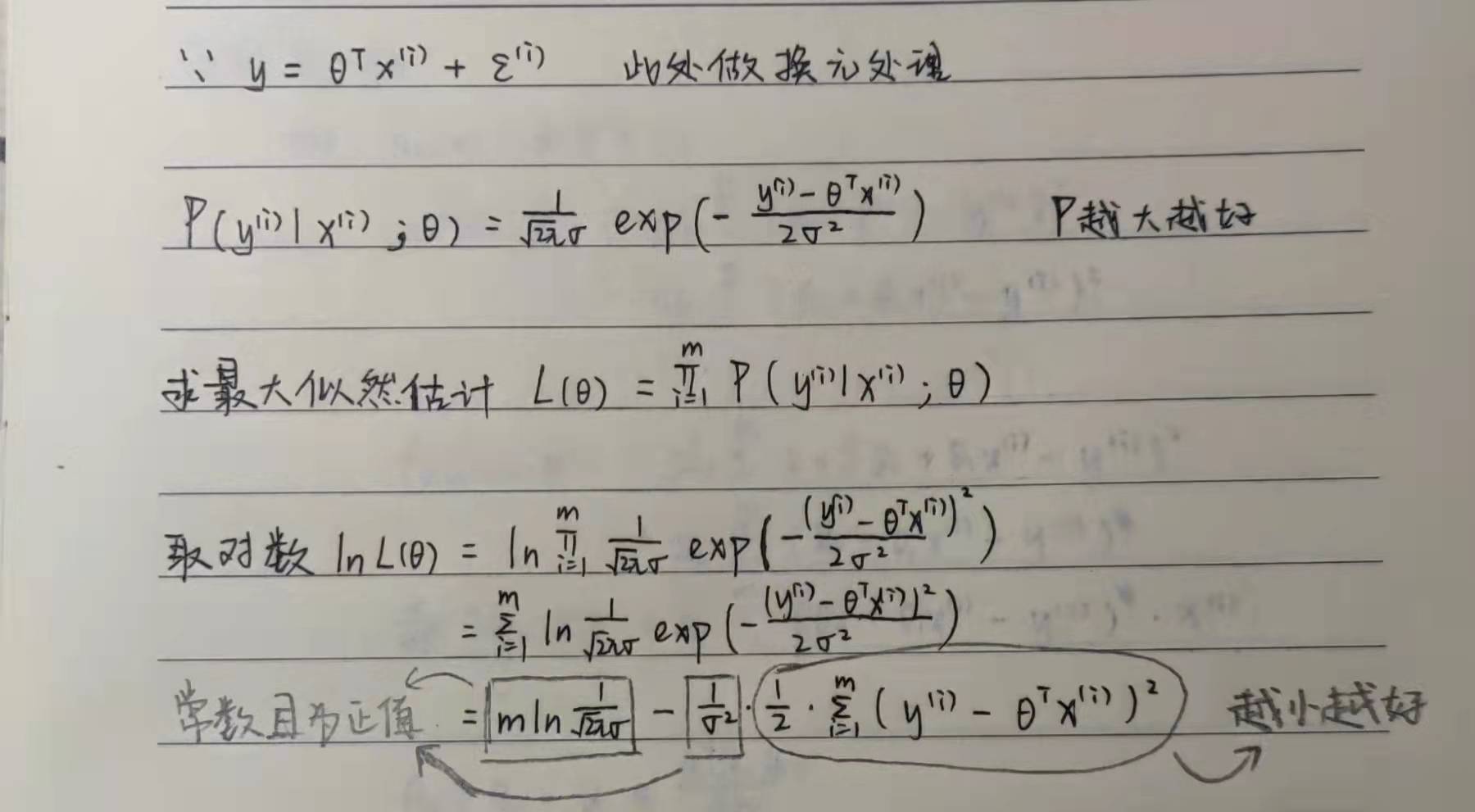
The knowledge of probability theory is applied here. We got the result in the last line. The purpose is to maximize P. obviously, we need to make the following formula as small as possible, so we get the mathematical concept of loss function:

 

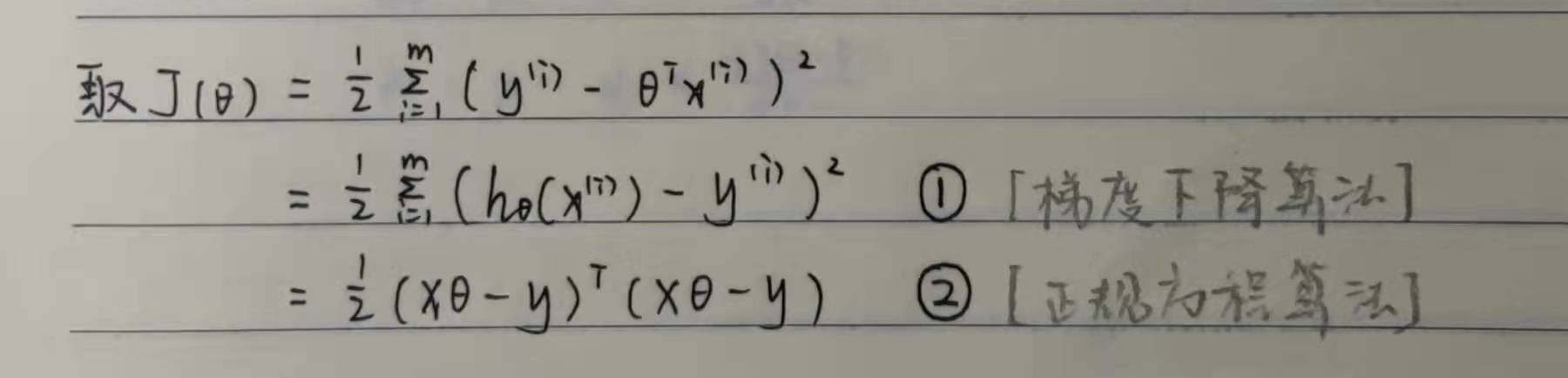
For whether we bring in the matrix operation, we get two different expressions, both of which can complete the calculation of the linear regression equation.

(1) Solving linear regression equation by gradient descent method

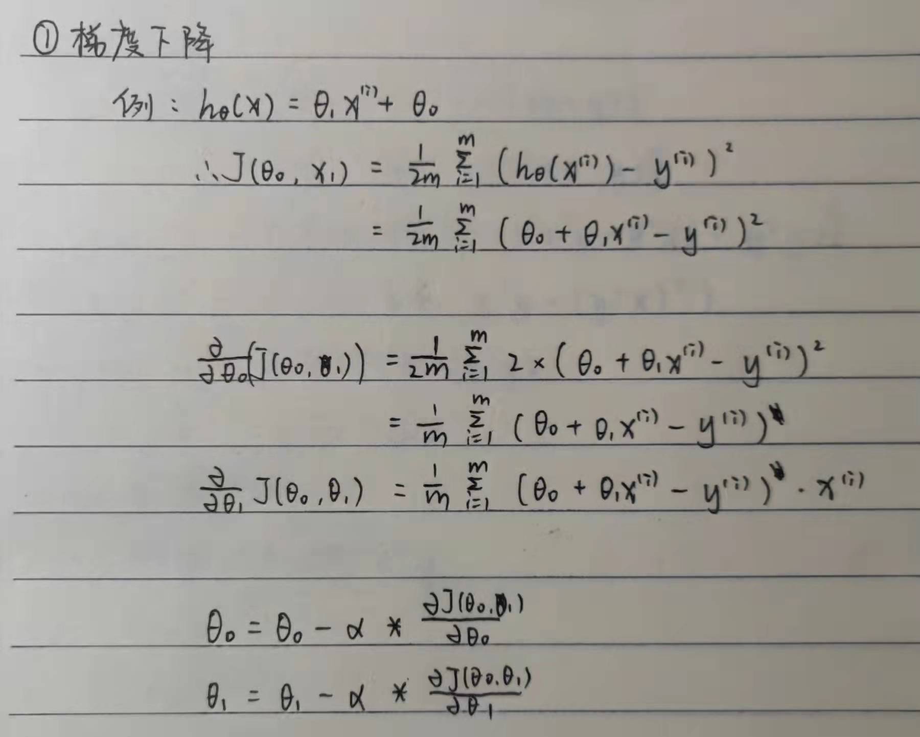
It should be noted that in the gradient descent algorithm, we need to define the step size alpha of each iteration. The size of alpha will affect the number of iterations and whether the maximum value of the loss function can be found. Usually, the number less than 1 is taken. Gradient descent algorithm has certain universality and can run normally when there are many parameters.

(2) Solving linear regression equation by normal equation method

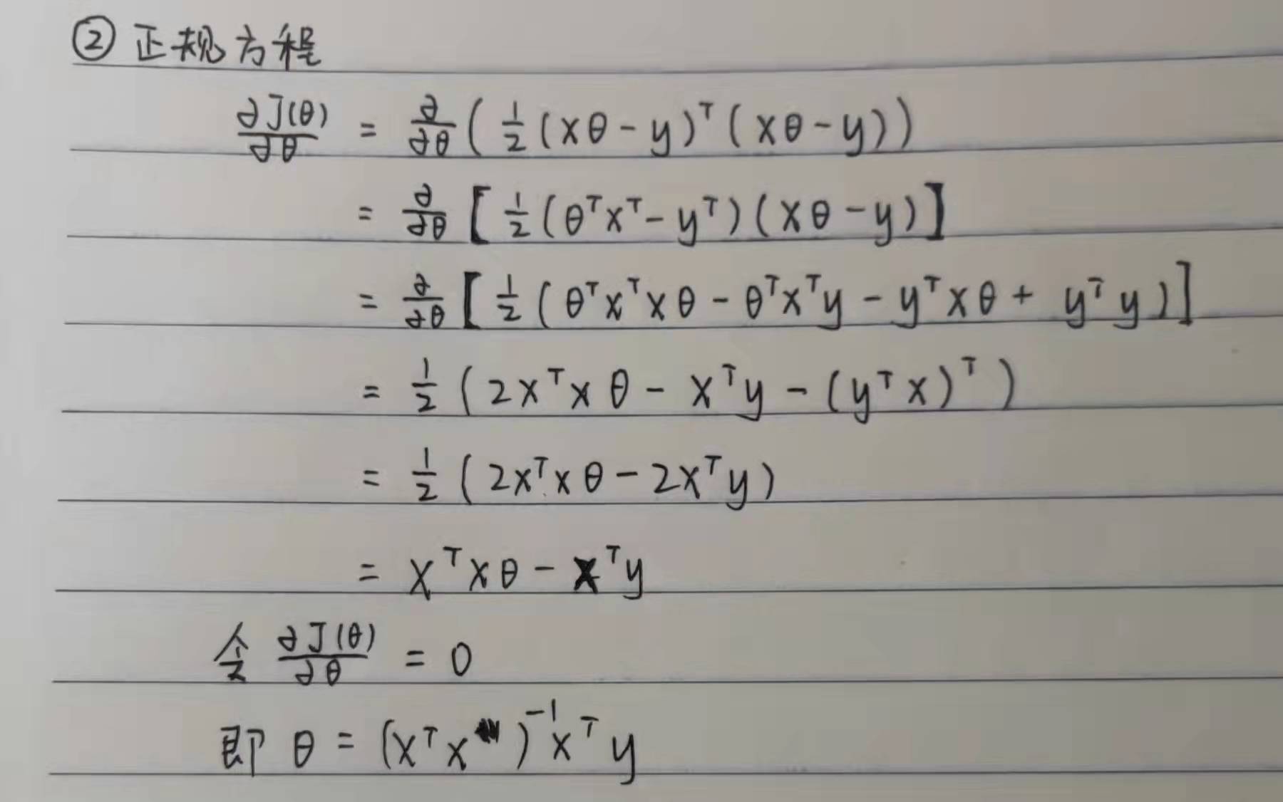
In the normal equation method, we can obtain the parameter theta without defining the size of step alpha and iteration. On the contrary, the normal equation needs to solve the transpose of the parameter x matrix. Even if the numpy function library can easily calculate the transpose matrix, the computation of the transpose matrix will reach a terrible order of magnitude when there are many parameters, so it is not universal.

2, Source code display

In the gradient descent algorithm, the number of parameters only involves the process of parameter derivation and parameter iteration, which is similar in principle. The author wrote the code in the notebook environment. The source code is shown below.

Import the necessary python libraries. We use pandas, numpy and matplotlib libraries.

import pandas as pd               #The pandas library is used to read data from csv tables
import numpy as np
import matplotlib.pyplot as plt

Define the function module for calculating the loss function and return the function value of the loss function.

#Find loss function
def Loss(theta0, theta1, theta2, x1, x2, y):
    h = theta0 + theta1 * x1 + theta2 * x2
    diff = h - y                        #At this point, h and y are both a 5-Dimensional matrix, and you can subtract directly to get each term and 
                                                  Difference between original values
    L = (diff.sum())**2 / (2 * x1.shape[0])    #x1.shape[0] gets the number of rows of the matrix, that is, in a 5-Dimensional matrix 
                                                      Indicates that there are several elements
    return L

Define the function module to calculate the partial derivative of each parameter to prepare for gradient descent.

#Finding the partial derivative of theta 0 in the loss function
def partial_loss_theta0(theta0, theta1, theta2, x1, x2, y):
    h = theta0 + theta1 * x1 + theta2 * x2
    diff = h - y                                       #The derivation process can use the formula derived above
    partial = diff.sum() / x1.shape[0]
    return partial

#Finding the partial derivative of theta 1 in the loss function
def partial_loss_theta1(theta0, theta1, theta2, x1, x2, y):
    h = theta0 + theta1 * x1 + theta2 * x2
    diff = (h - y) * x1                               #The derivation process can use the formula derived above
    partial = diff.sum() / x1.shape[0]
    return partial

#Finding the partial derivative of theta 2 in the loss function
def partial_loss_theta2(theta0, theta1, theta2, x1, x2, y):
    h = theta0 + theta1 * x1 + theta2 * x2
    diff = (h - y) * x2                               #The derivation process can use the formula derived above
    partial = diff.sum() / x1.shape[0]
    return partial

The core algorithm of gradient descent is as follows.

#Finding the minimum point of loss function by gradient descent
def gradient_descent(x1, x2, y, alpha=0.1, theta0 = 1, theta1 = 1, theta2 = 1, steps = 5000):
    num = 0                   #Number of iterations
    result=[]
    for step in range(steps):
        num += 1
        update0 = partial_loss_theta0(theta0, theta1, theta2, x1, x2, y)
        update1 = partial_loss_theta1(theta0, theta1, theta2, x1, x2, y)
        update2 = partial_loss_theta2(theta0, theta1, theta2, x1, x2, y)
        
        theta0 = theta0 - alpha * update0                  #The three parameters are iterated at the same time
        theta1 = theta1 - alpha * update1
        theta2 = theta2 - alpha * update2
        
        e = Loss(theta0, theta1, theta2, x1, x2, y)
        result.append(e)
        if e < 0.001:
            break
    
    return theta0,theta1,theta2,result

Here, the author uses the feature scaling of data to make the data more centralized and regular, so as to greatly improve the operation speed. Attached here is the result display of data standardization on the notebook:

ranges = pd.read_csv("ranges.csv")
ranges.Salary = (ranges.Salary - ranges.Salary.mean()) / ranges.Salary.std() #The original data is standardized here
ranges.Age = (ranges.Age - ranges.Age.mean()) / ranges.Age.std()        #The standardized data will greatly reduce the number of operations
ranges.Range = (ranges.Range - ranges.Range.mean()) / ranges.Range.std()
ranges                                                   #Display of results after data standardization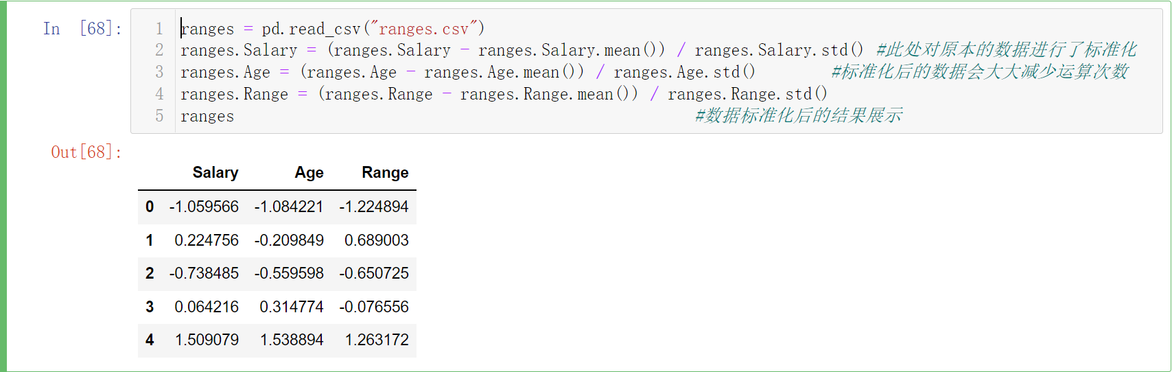

Finally, the main function is defined, and the gradient descent image of the loss function is drawn by matplotlib

if __name__ == "__main__":
    theta0,theta1,theta2,result = gradient_descent(ranges.Salary, ranges.Age, ranges.Range)
    print("\n The linear programming equation is:\n")
    print("h(x) = %.3f + %.3f * x1 + %.3f * x2\n"%(theta0,theta1,theta2))
    n = len(result)
    x = range(n)
    plt.plot(x,result,color='r',linewidth=3)
    plt.title("Loss")
    plt.xlabel("num")
    plt.ylabel("y")
    plt.show()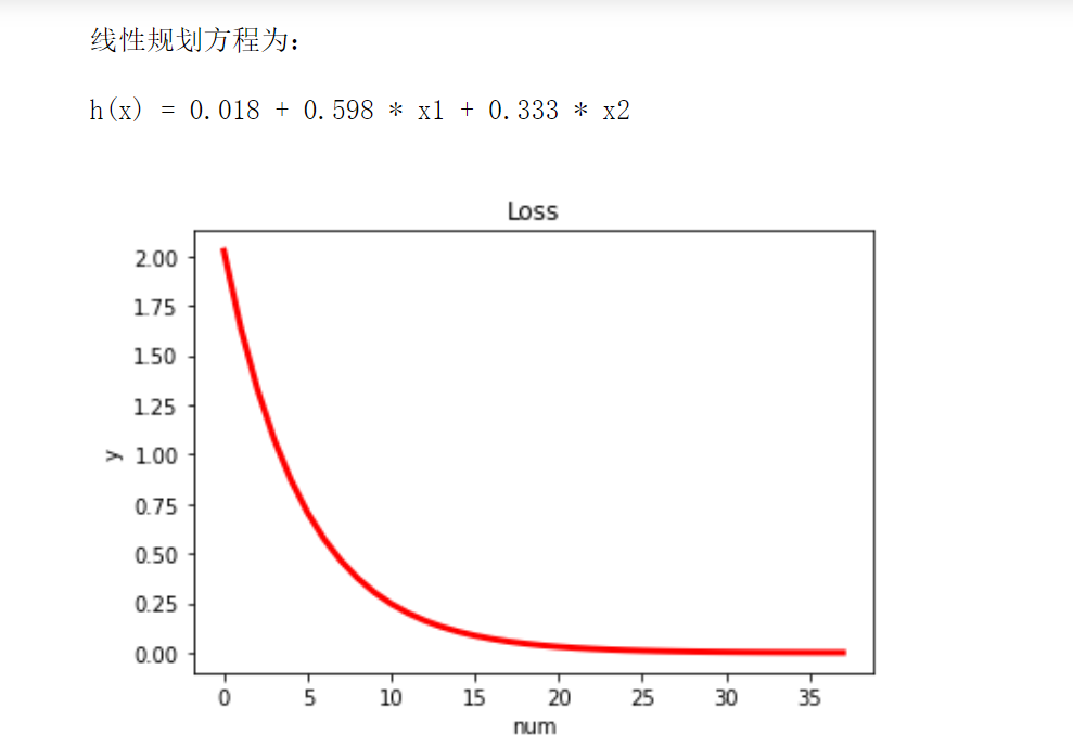

 

We can see that the standardized data can basically fit a better prediction function after about 30 calculations, with high efficiency.