• summary:
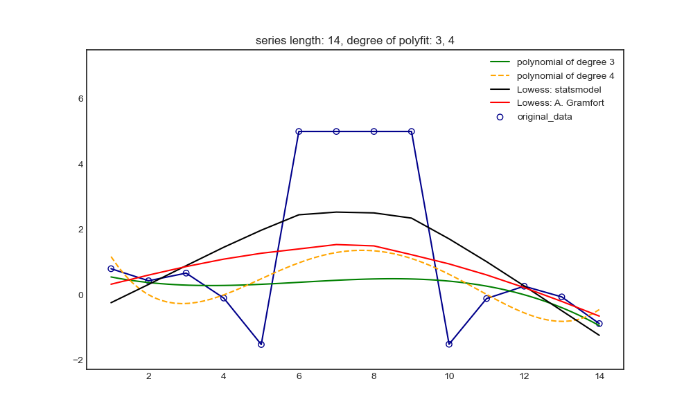
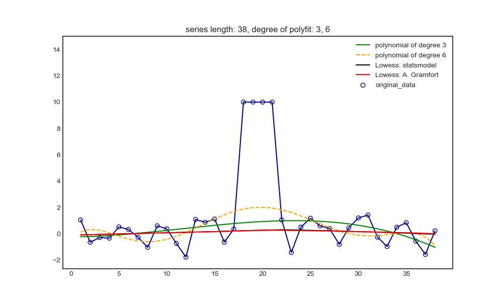
  1. When calculating the effect coefficient of outlier interval in the sequence, such as holiday coefficient, the increased non outlier interval on the left and right sides should be as long as possible. The stronger the degree of outlier, the longer the increased non outlier interval,
  Polynomial and Lowess can not be pulled up. Since the pulling degree cannot be accurately controlled, it is better not to pull up uniformly.
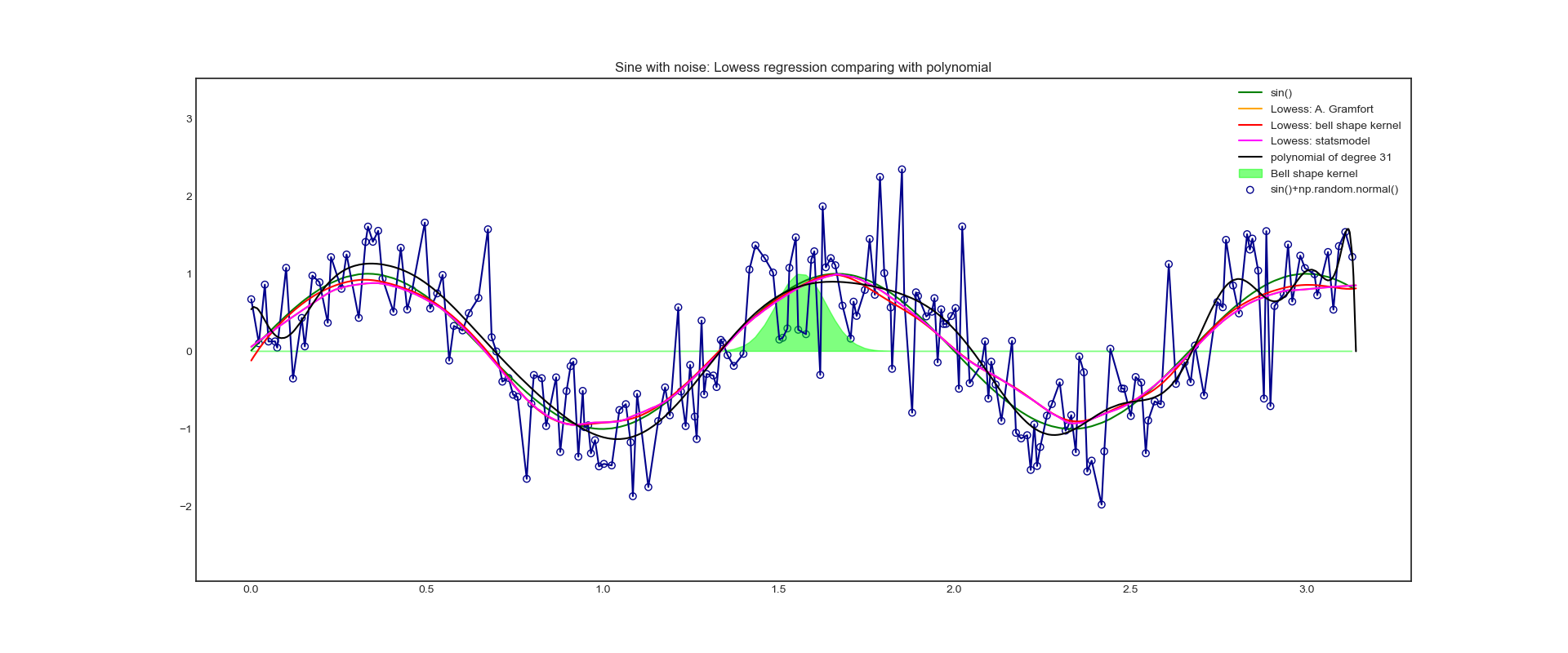
  2. When it is necessary to learn the basic laws of the sequence, the polynomial can be as large as possible (it will not oscillate at the fitting independent variable point), and Lowess is a large frac and it.

• Explanation:

• For Polynomials:
  1. (especially important) when the polynomial fitting degree is too high, the new dependent variable will oscillate in the interval except the original independent variable points, so when applying the fitted polynomial, the new independent variable cannot fall in these intervals,
  However, if it falls on any original independent variable point, it will never oscillate. That is, although the higher the degree, the more the polynomial will be over fitted, if the new independent variable falls on the point of the original independent variable, the new dependent variable will only approach the value of the original dependent variable,
  But it will never oscillate.
  When the fitting times are low, it is not easy to oscillate in all intervals and independent variable points, and the function has poor follow-up and strong regularity. When the new independent variable falls on the original independent variable point, the new dependent variable will also deviate far from the cause variable.
  Therefore, when the value of the new strain does not exceed the set of the original independent variables, the fitting times can be appropriately higher, because there is no need to worry about oscillation; If the fitting times are low, the new strain will deviate further from the original strain, which is less conducive to reflect the basic law.
  2. When the fitting times are high, the polynomial is easy to oscillate at both ends or one end and more outside of the independent variable interval during fitting. When the dependent variable in the middle interval is taken, it can not oscillate.
  3. When there are too many fitting points and the degree is high, the singular value decomposition does not converge when doing the least squares, so the polynomial cannot be fitted.
  When there are few fitting points, the fitting times can exceed the fitting points, that is, the number of unknowns exceeds the number of equations. Although the unknowns cannot be obtained by solving the linear equations, the unknowns can be obtained by optimization methods such as gradient descent,
  That is, the coefficients of polynomials. At this time, it is easy to oscillate, and the non oscillation interval in the middle is narrower.

• For locally weighted regression:
  1. The LOWESS method returns the fitting value instead of the function, so the return value corresponds to the independent variable x one by one, and cannot get the more dense or sparse return value or the return value outside the independent variable interval.
  2. The closer frac is to 1, the closer fitting sliding window is to the full length, and the smoother regression value is, but frac cannot be greater than 1; The larger the it number, the more the nearest points to recalculate the weight, and the less affected by the nearest outliers;
  Because it is already relatively smooth at this time, the number of it required is small.
  3. The closer frac is to 0, the fewer the nearest samples in the fitting sliding window, the stronger the follow-up of regression value and the worse the regularity; Because the number of it should not be greater than the number of samples in the sliding window, the number of it should also be small at this time.
  4. When there are outliers in the sequence, the IT value can be taken as the number of samples in the longest outlier + 1, so that no matter which Lowess method is used, it will not be affected by the outliers.

• Practice:

from math import ceil
import numpy as np
from scipy import linalg
import statsmodels.api as sm
import matplotlib.pyplot as plt
import copy
plt.style.use('seaborn-white')


# Defining the bell shaped kernel function - used for plotting later on
def kernel_function(xi, x0, tau=.005):
    return np.exp(- (xi - x0) ** 2 / (2 * tau))


def lowess_bell_shape_kern(x, y, tau=.005):
    """
    lowess_bell_shape_kern(x, y, tau = .005) -> yest
    Locally weighted regression: fits a nonparametric regression curve to a scatterplot.
    The arrays x and y contain an equal number of elements; each pair
    (x[i], y[i]) defines a data point in the scatterplot. The function returns
    the estimated (smooth) values of y.
    The kernel function is the bell shaped function with parameter tau. Larger tau will result in a
    smoother curve.
    """
    n = len(x)
    yest = np.zeros(n)

    # Initializing all weights from the bell shape kernel function
    w = np.array([np.exp(- (x - x[i]) ** 2 / (2 * tau)) for i in range(n)])

    # Looping through all x-points
    for i in range(n):
        weights = w[:, i]
        b = np.array([np.sum(weights * y), np.sum(weights * y * x)])
        A = np.array([[np.sum(weights), np.sum(weights * x)],
                      [np.sum(weights * x), np.sum(weights * x * x)]])
        theta = linalg.solve(A, b)
        yest[i] = theta[0] + theta[1] * x[i]

    return yest


def lowess_ag(x, y, frac=2/3, it=3):
    """
    lowess(x, y, frac=2./3., it=3) -> yest
    Lowess smoother: Robust locally weighted regression.
    The lowess function fits a nonparametric regression curve to a scatterplot.
    The arrays x and y contain an equal number of elements; each pair
    (x[i], y[i]) defines a data point in the scatterplot. The function returns
    the estimated (smooth) values of y.
    The smoothing span is given by frac. A larger value for frac will result in a
    smoother curve. The number of robustifying iterations is given by it. The
    function will run faster with a smaller number of iterations.
    """
    n = len(x)
    r = int(ceil(frac * n))
    h = [np.sort(np.abs(x - x[i]))[r] for i in range(n)]
    w = np.clip(np.abs((x[:, None] - x[None, :]) / h), 0.0, 1.0)
    w = (1 - w ** 3) ** 3
    yest = np.zeros(n)
    delta = np.ones(n)
    for iteration in range(it):
        for i in range(n):
            weights = delta * w[:, i]
            b = np.array([np.sum(weights * y), np.sum(weights * y * x)])
            A = np.array([[np.sum(weights), np.sum(weights * x)],
                          [np.sum(weights * x), np.sum(weights * x * x)]])
            beta = linalg.solve(A, b)
            yest[i] = beta[0] + beta[1] * x[i]

        residuals = y - yest
        s = np.median(np.abs(residuals))
        delta = np.clip(residuals / (6.0 * s), -1, 1)
        delta = (1 - delta ** 2) ** 2

    return yest


lowess_sm = sm.nonparametric.lowess
tau = 0.005  # The larger the abs(tau), the lower_ bell_ shape_ The smoother the regression value of Kern; Tau → 0 +, the stronger the follow-up of regression value, the worse the regularity.
samples_in_window = 24  # samples_ in_ The closer the window is to the total number of samples, the smoother the regression value is; The closer to 1, the stronger the follow-up of regression value and the worse the regularity.
frac = 0.9
n = 31  # The highest degree of polynomial, and there are n+1 unknowns (variables to be fitted)

# Test the first sinusoidal data set
scale = 5
x_plot = np.random.uniform(low=0, high=1*np.pi, size=200*scale)
x_plot.sort()
y_plot = np.sin(x_plot * 1.5 * np.pi)
y_noise_plot = y_plot + np.random.normal(scale=1/2, size=len(x_plot))
x = np.array([x_plot[5*i] for i in range(int(len(x_plot)/scale))])
y = np.sin(x * 1.5 * np.pi)
y_noise = y + np.random.normal(scale=1/2, size=len(x))

# The loss method returns the fitting value instead of the function, so the return value corresponds to the independent variable x one by one, and cannot get a more dense or sparse return value
yest_bell_plot = lowess_bell_shape_kern(x_plot, y_noise_plot, tau=tau)
# The closer the frac is to 1, the closer the fitting sliding window is to the full length, and the smoother the regression value is; The larger the IT number, the more the nearest points to recalculate the weight, and the less affected by the nearest outliers; Because it is already relatively smooth at this time, the number of it required is small.
# The closer frac is to 0, the fewer the nearest samples in the fitting sliding window, the stronger the follow-up of regression value and the worse the regularity; Because the number of it should not be greater than the number of samples in the sliding window, the number of it should also be small at this time.
yest_ag_plot = lowess_ag(x_plot, y_noise_plot, frac=samples_in_window/len(x), it=3)
yest_sm_plot = lowess_sm(y_noise_plot, x_plot, frac=samples_in_window/len(x), it=3, return_sorted=False)
# polyfit and poly1d return function p, so assigning any x to this function p can get the corresponding dependent variable y
c = np.polyfit(x, y_noise, n)
p = np.poly1d(c)
y_poly_plot = p(x_plot)

# plot to compare three kinds of Lowess method
plt.figure(figsize=(20, 8))
plt.plot(x, y, color='g', label='sin()')
plt.scatter(x, y_noise, facecolors='none', edgecolor='darkblue', label='sin()+np.random.normal()')
plt.plot(x, y_noise, color='darkblue')
plt.fill(x[:], kernel_function(x[:], max(x)/2, tau), color='lime', alpha=0.5, label='Bell shape kernel')
plt.plot(x_plot, yest_ag_plot, color='orange', label='Lowess: A. Gramfort')
plt.plot(x_plot, yest_bell_plot, color='red', label='Lowess: bell shape kernel')
plt.plot(x_plot, yest_sm_plot, color='magenta', label='Lowess: statsmodel')
plt.plot(x_plot, y_poly_plot, color='k', label='polynomial of degree {}'.format(n))
plt.ylim(min(y_noise) - abs(min(y_noise) / 2), max(y_noise) * 1.5)  # Make the upper and lower limits of y coordinate symmetrical about the maximum and minimum value of y, and not affected by the oscillation value of polynomial fitting function
plt.legend()
plt.title('Sine with noise: Lowess regression comparing with polynomial')


# Test the second dataset with outliers
x = [np.linspace(1, 14, 14), np.linspace(1, 38, 38)]
# x_plot makes the value of X in drawing more intensive than that in polynomial fitting, so as to observe the possible oscillation
x_plot = [np.linspace(1, int(max(x[0])), int(max(x[0]))*5), np.linspace(1, int(max(x[1])), int(max(x[1]))*5)]
y = [np.random.randn(len(x[0])), np.random.randn(len(x[1]))]
# Set outliers
for i in range(len(x)):
    y[i][int(len(x[i])/2-2):int(len(x[i])/2+2)] = 5*(i+1)
n = [[3, 4], [3, 6]]
weights = [(max(y[i])*2-y[i])/sum(max(y[i])*2-y[i]) for i in range(len(x))]  # The larger y[i], the smaller the weights; Let outliers account for less weight and normal points account for more weight.

c = copy.deepcopy(n)  # c and n have the same structure; Be sure to use copy Deep copy, shallow copy cannot be used, otherwise the subsequent assignment to c will also change n
p = copy.deepcopy(n)  # p and n have the same structure
yest_sm, yest_ag = [], []
for i in range(len(x)):
    for j in range(len(n[i])):
        c[i][j] = np.polyfit(x[i], y[i], n[i][j], full=True, w=weights[i])
        p[i][j] = np.poly1d(c[i][j][0])
        print('Sequence length{0}Points, fitting times{1}，That is, the number of unknowns of the objective function is{2}，That is, the number of equations for the partial derivative of the objective function to the independent variable is{2}: '.format(len(x[i]), n[i][j], n[i][j]+1))
        print('Coefficient of fitting function (from high to low):', '\n', c[i][j][0])
        print('Comparison between fitting value and actual value MAPE: ', sum(abs((p[i][j](x[i])-y[i])/y[i]))/len(x[i]))
        print('Rank of coefficient matrix of objective function to independent variable partial derivative equations:', c[i][j][2])
        print('Singular value of coefficient matrix of objective function to independent variable partial derivative equations:', '\n', c[i][j][3])
        print('Number of relevant conditions for fitting:', c[i][j][4], '\n')
    plt.figure(figsize=(10, 6))
    plt.scatter(x[i], y[i], facecolors='none', edgecolor='darkblue', label='original_data')
    plt.plot(x[i], y[i], color='darkblue')
    plt.plot(x_plot[i], p[i][0](x_plot[i]), '-', color='g', label='polynomial of degree {}'.format(n[i][0]))
    plt.plot(x_plot[i], p[i][1](x_plot[i]), '--', color='orange', label='polynomial of degree {}'.format(n[i][1]))
    yest_sm.append(lowess_sm(y[i], x[i], frac=frac, it=5, return_sorted=False))
    yest_ag.append(lowess_ag(x[i], y[i], frac=frac, it=5))
    plt.plot(x[i], yest_sm[i], color='k', label='Lowess: statsmodel')
    plt.plot(x[i], yest_ag[i], color='r', label='Lowess: A. Gramfort')
    plt.ylim(min(y[i])-abs(min(y[i])/2), max(y[i])*1.5)  # Make the upper and lower limits of y coordinate symmetrical about the maximum and minimum value of y, and not affected by the oscillation value of polynomial fitting function
    plt.legend()
    plt.title('series length: {0}, degree of polyfit: {1}, {2}'.format(len(x[i]), n[i][0], n[i][1]))

• Graphic display:
  sin()+noise: polynomial and Lowess can learn better
  
  The shorter non outlier intervals on both sides: polynomial and Lowess are pulled up
  
  Longer non outlier intervals on both sides: polynomial and Lowess can not be pulled up