Text / Zaid Alyafeai
We will create a simple tool to identify the drawing and output the name of the current drawing. This application will run directly on the browser without any installation. We will use Google lab to train the model and tensorflow JS deploy it in the upper part of the browser.
[to get TensorFlow js. Video tutorial, please go to Bilibili, TensorFlow channel: https://www.bilibili.com/video/BV1D54y1p7PQ]
Code and demonstration
Find the live demo and code on GitHub. Also, be sure to test the notebook on Google Colab here.
Note: link here
data set
We will use CNN to identify different types of patterns. CNN will train on the Quick Draw dataset. The dataset contains about 345 categories and 50 million patterns.
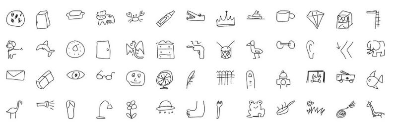
Subset of class
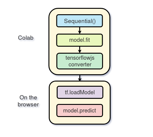
Transmission pathway
We will use Keras to train the model for free on the GPU of Google Colab, and then use tensorflow JS (tfjs) runs directly on the browser. I'm at tensorflow JS, please read it before continuing. This is the delivery route of the project:
Training at Colab
Google offers free processing power on the GPU. You can see how to create a notebook and activate GPU Programming in this tutorial.
input
We will use keras based on tensorflow
1    import os

2    import glob

3    import numpy as np

4    from tensorflow.keras import layers

5    from tensorflow import keras

6    import tensorflow as tf
Load data
Due to limited memory, we will not train all categories. We only use 100 data sets. The data of each category can be used as a numpy array with the shape [N, 784] on Google Cloud, where N is the number of images of that specific category. Let's first download the dataset
1    import urllib.request

2    def download():

3

4        base = 'https://storage.googleapis.com/quickdraw_dataset/full/numpy_bitmap/'

5        for c in classes:

6            cls_url = c.replace('_', '%20')

7            path = base+cls_url+'.npy'

8            print(path)

9            urllib.request.urlretrieve(path, 'data/'+c+'.npy')
Due to the limited memory, we will only load 5000 images in each category into memory. 20% of untested data is also retained
1    def load_data(root, vfold_ratio=0.2, max_items_per_class= 5000 ):

2        all_files = glob.glob(os.path.join(root, '*.npy'))

3

4        #initialize variables

5        x = np.empty([0, 784])

6        y = np.empty([0])

7        class_names = []

8

9        #load a subset of the data to memory

10        for idx, file in enumerate(all_files):

11            data = np.load(file)

12            data = data[0: max_items_per_class, :]

13            labels = np.full(data.shape[0], idx)

14

15            x = np.concatenate((x, data), axis=0)

16            y = np.append(y, labels)

17

18            class_name, ext = os.path.splitext(os.path.basename(file))

19            class_names.append(class_name)

20

21        data = None

22        labels = None

23

24        #separate into training and testing

25        permutation = np.random.permutation(y.shape[0])

26        x = x[permutation, :]

27        y = y[permutation]

28

29        vfold_size = int(x.shape[0]/100*(vfold_ratio*100))

30

31        x_test = x[0:vfold_size, :]

32        y_test = y[0:vfold_size]

33

34        x_train = x[vfold_size:x.shape[0], :]

35        y_train = y[vfold_size:y.shape[0]]

return x_train, y_train, x_test, y_test, class_names
Preprocessing data
We preprocessed the data and prepared to start training.
1    # Reshape and normalize

2    x_train = x_train.reshape(x_train.shape[0], image_size, image_size, 1).astype('float32')

3    x_test = x_test.reshape(x_test.shape[0], image_size, image_size, 1).astype('float32')

4

5    x_train /= 255.0

6    x_test /= 255.0

7

8    # Convert class vectors to class matrices

9    y_train = keras.utils.to_categorical(y_train, num_classes)

10    y_test = keras.utils.to_categorical(y_test, num_classes)
Create model
We will create a simple CNN. Note that the smaller the number of parameters, the simpler the model, the better. In fact, we will run the model after the browser conversion, and we want the model to run quickly and predict. The following model contains 3 conversion layers and 2 dense layers.
1    # Define model

2    model = keras.Sequential()

3    model.add(layers.Convolution2D(16, (3, 3),

4                            padding='same',

5                            input_shape=x_train.shape[1:], activation='relu'))

6    model.add(layers.MaxPooling2D(pool_size=(2, 2)))

7    model.add(layers.Convolution2D(32, (3, 3), padding='same', activation= 'relu'))

8    model.add(layers.MaxPooling2D(pool_size=(2, 2)))

9    model.add(layers.Convolution2D(64, (3, 3), padding='same', activation= 'relu'))

10    model.add(layers.MaxPooling2D(pool_size =(2,2)))

11    model.add(layers.Flatten())

12    model.add(layers.Dense(128, activation='relu'))

13    model.add(layers.Dense(100, activation='softmax'))

14    # Train model

15    adam = tf.train.AdamOptimizer()

16    model.compile(loss='categorical_crossentropy',

17                    optimizer=adam,

18                    metrics=['top_k_categorical_accuracy'])

19    print(model.summary())
Adaptation, verification and testing
After that, we based on 5 epochs and 256 batch training models.
1    #fit the model

2    model.fit(x = x_train, y = y_train, validation_split=0.1, batch_size = 256, verbose=2, epochs=5)

3

4    #evaluate on unseen data

5    score = model.evaluate(x_test, y_test, verbose=0)

6    print('Test accuarcy: {:0.2f}%'.format(score[1] * 100))
Here are the results of the training
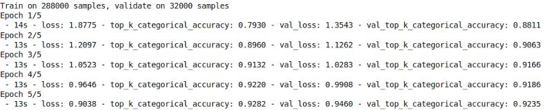
The test accuracy is 92.20%.
Preparing models in Web format
After we are satisfied with the accuracy of the model, we save it for conversion
1 model.save('keras.h5')We installed the tfjs package for conversion
1 !pip install tensorflowjs
Then we transform the model
1    !mkdir model

2    !tensorflowjs_converter --input_format keras keras.h5 model/
This creates some weight files and json files that contain the model architecture.
Compress the model and prepare to download it to your local computer
1 !zip -r model.zip model
Finally, download the model
1    from google.colab import files

2    files.download('model.zip')
Browser inference
In this section, we will show how to load the model and reason. Suppose we have a canvas with a size of 300 x 300. About interface and tensorflow I won't expand the JS part one by one.
Loading model
To use tensorflow JS first, we use the following script
1 <script src="https://cdn.jsdelivr.net/npm/@tensorflow/tfjs@latest"> </script>
You need to run the server on the local computer to host the weight file. Like me, you can create an apache server on the project or host pages on GitHub.
After that, load the model into the browser
1 model = await tf.loadModel('model/model.json')Use await to wait for the browser to load the model.
Pretreatment
We need to preprocess the data before making predictions. First, get the image data from the canvas
1    //the minimum boudning box around the current drawing

2    const mbb = getMinBox()

3    //cacluate the dpi of the current window

4    const dpi = window.devicePixelRatio

5    //extract the image data

6    const imgData = canvas.contextContainer.getImageData(mbb.min.x * dpi, mbb.min.y * dpi,

7                                                (mbb.max.x - mbb.min.x) * dpi, (mbb.max.y - mbb.min.y) * dpi);
We'll explain getMinBox() later. The variable dpi is used to stretch the canvas according to the density of screen pixels.
We convert the current image data of the canvas into tensors, resize and standardize.
1    function preprocess(imgData)

2    {

3    return tf.tidy(()=>{

4            //convert the image data to a tensor

5            let tensor = tf.fromPixels(imgData, numChannels= 1)

6            //resize to 28 x 28

7            const resized = tf.image.resizeBilinear(tensor, [28, 28]).toFloat()

8            // Normalize the image

9            const offset = tf.scalar(255.0);

10        const normalized = tf.scalar(1.0).sub(resized.div(offset));

11            //We add a dimension to get a batch shape

12            const batched = normalized.expandDims(0)

13            return batched

14    })

15    }
For prediction, we use model Predict this returns the probability that the shape is [N, 100].
1 const pred = model.predict(preprocess(imgData)).dataSync()
Then we can use a simple function to find the first five probabilities.
Improve accuracy
Remember that our model accepts tensors with the shape [N, 28,28,1]. Our drawing canvas size is 300 x 300, which may be too large for drawing, or users may want to draw a small picture. The box containing the current drawing is clipped to the best size. To this end, we extract the minimum bounding box around the graph by looking at the upper left corner and the lower right corner
1 //record the current drawing coordinates
2 function recordCoor(event)
3 {
4 //get current mouse coordinate
5 var pointer = canvas.getPointer(event.e);
6 var posX = pointer.x;
7 var posY = pointer.y;
8
9 //record the point if withing the canvas and the 10 mouse is pressed
if(posX >=0 && posY >= 0 && mousePressed)
11 {
12 coords.push(pointer)
13 }
14 }
15
16 //get the best bounding box by finding the top left and bottom right cornders
17 function getMinBox(){
18
19 var coorX = coords.map(function(p) {return p.x});
20 var coorY = coords.map(function(p) {return p.y});
21 //find top left corner
22 var min_coords = {
23 x : Math.min.apply(null, coorX),
24 y : Math.min.apply(null, coorY)
25 }
26 //find right bottom corner
27 var max_coords = {
28 x : Math.max.apply(null, coorX),
29 y : Math.max.apply(null, coorY)
30 }
31 return {
32 min : min_coords,
33 max : max_coords
34 }
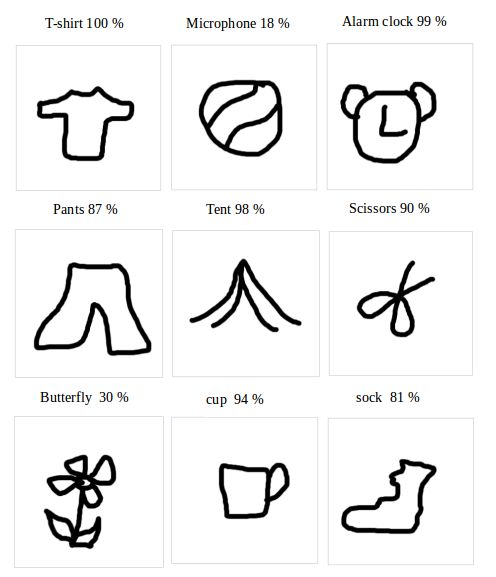
35 } Test drawing
The following are the most frequent patterns in your first drawing. I drew all the drawings with the mouse. If you use a pen, the accuracy will be higher.
Want to know about TensorFlow js For more practical cases of components, please go to bilibilibili Google China TensorFlow channel to view Made With TensorFlow js Chinese series video.
https://www.bilibili.com/video/BV1D54y1p7PQ
For more information about TensorFlow, please visit TensorFlow's official website in China( tensorflow.google.cn ) check or scan the two-dimensional code below, and pay attention to the TensorFlow official account.