1, Introduction

Target tracking is a technology that uses the information about the target obtained by various types of sensors to estimate and predict the real state and future state of the target. Target tracking technology is widely used in military and civil fields. With the progress of electronic technology and computer technology, a variety of new technologies and theories have been applied to the field of target tracking. Target tracking technology has gradually developed into an interdisciplinary, cross industry and multi-level technology. The main content of target tracking technology is to accurately estimate and predict the real information of the target from the imprecise information about the target obtained from the sensor. Therefore, various filters are needed to filter the collected data. As a filtering algorithm with excellent performance, Kalman filter has been widely used in the field of target tracking, but the filter is based on a certain target tracking model. Therefore, the research object of target tracking mainly includes tracking model and filtering algorithm. In these two aspects, many scholars at home and abroad have conducted in-depth research and achieved fruitful results. As a new data fusion algorithm, interactive multi model (IMM) algorithm has been paid enough attention in recent years because of its excellent tracking effect and wide tracking frequency band

2, Source code

%**********utilize Singer The model algorithm tracks the maneuvering target*************
function [xx5,yy5,ex5,exv5]=singer(T,r,N)
clc
clear
close all
% %***************Simulation conditions********************
T=2;      %Radar scanning cycle
r=10000;  %Measurement error variance
N=50;%Monte Carlo Simulation times
%alpha=1/60;%The reciprocal of the maneuver time constant, that is, the maneuver frequency
F=[1 T (1/2)*T^2 0 0 0;
   0 1 T  0 0 0;
   0 0 1  0 0 0;
   0 0 0  1 T (1/2)*T^2; 
   0 0 0  0 1 T;
   0 0 0  0 0 1];%State transition matrix
H=[1 0 0 0 0 0;
   0 0 0 1 0 0];%Measurement matrix
sigmax=r;%X Directional measurement noise variance
sigmay=r;%Y Directional measurement noise variance
R=[sigmax 0;
   0 sigmay];%Measurement noise covariance
%sigmaax=0.01;%X Directional target acceleration variance
%sigmaay=0.01;%Y Directional target acceleration variance
qq11=T^5/20;
qq12=T^4/8;
qq13=T^3/6;
qq22=T^3/3;
qq23=T^2/2;
qq33=T;
qq44=T^5/20;
qq45=T^4/8;
qq46=T^3/6;
qq55=T^3/3;
qq56=T^2/2;
qq66=T;
Q=[qq11 qq12 qq13 0    0    0;
   qq12 qq22 qq23 0    0    0;
   qq13 qq23 qq33 0    0    0;
   0    0    0    qq44 qq45 qq46;
   0    0    0    qq45 qq55 qq56;
   0    0    0    qq46 qq56 qq66];%process noise covariance 
for j=1:N
    [x,y,zx,zy,NN]=target_movement;
    load target_movement_out
    z=[zx';zy'];
    X=[z(1,3) (z(1,3)-z(1,2))/T (z(1,3)-2*z(1,2)+z(1,1))/T^2 z(2,3) (z(2,3)-z(2,2))/T (z(2,3)-2*z(2,2)+z(2,1))/T^2]';%State vector initialization
    %Filter covariance initialization
    P11=R(1,1);
    P12=R(1,1)/T;
    P13=R(1,1)/T^2;
    P22=2*R(1,1)/T^2;
    P23=3*R(1,1)/T^3;
    P33=6*R(1,1)/T^4;
    P44=R(2,2);
    P45=R(2,2)/T;
    P46=R(2,2)/T^2;
    P55=2*R(2,2)/T^2;
    P56=3*R(2,2)/T^3;
    P66=6*R(2,2)/T^4;
    P=[P11 P12 P13 0   0   0;
        P12 P22 P23 0   0   0;
        P13 P23 P33 0   0   0;
        0   0   0   P44 P45 P46;
        0   0   0   P45 P55 P56;
        0   0   0   P46 P56 P66];
    MX(:,3)=X; 
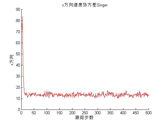
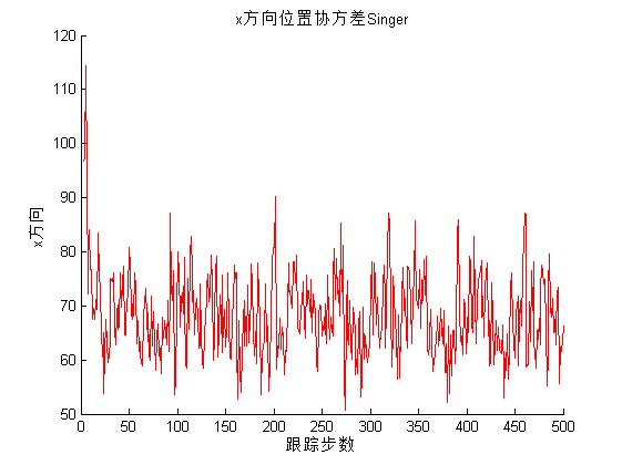
    EX(j,3)=(X(1)-x(3)).^2;%x Direction position initial variance
    EXv(j,3)=(X(2)-vvx(3)).^2;%x Initial variance of directional velocity
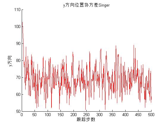
    EY(j,3)=(X(4)-y(3)).^2;%y Direction position initial variance
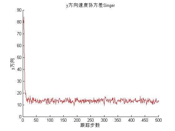
    EYv(j,3)=(X(5)-vvy(3)).^2;%y Initial variance of directional velocity
    for i=4:NN
        x1=F*X;
        z1=H*x1;
        P1=F*P*F'+Q;
        S=H*P1*H'+R;
        v=z(:,i)-z1;
        W=P1*H'*inv(S);
        X=x1+W*v;
        P=P1-W*S*W';
        Mv=v'*inv(S)*v;
        MX(:,i)=X;
        MEX(:,i,j)=MX(:,i);
        EX(j,i)=(X(1)-x(i)).^2;%x Direction position initial variance
        EXv(j,i)=(X(2)-vvx(i)).^2;%x Initial variance of directional velocity
        EY(j,i)=(X(4)-y(i)).^2;%y Direction position initial variance
        EYv(j,i)=(X(5)-vvy(i)).^2;%x Initial variance of directional velocity        
    end
end
function [x,y,zx,zy,NN]=target_movement
%Function definition: generate the real value and measured value of the target motion
% %***************Simulation conditions*******************************************************
T=2;      %Radar scanning cycle
r=10000;  %Measurement error variance
x0=2000;%Target in X Starting position in axis direction
y0=10000;%Target in Y Starting position in axis direction
xv0=0;%Target in X Initial speed in axis direction
yv0=-15;%Target in Y Initial speed in axis direction
NN=500;%Sampling points
x=zeros(NN,1);%X Axis position initialization
y=zeros(NN,1);%Y Axis position initialization
x(1)=x0;%X Axis initial position
y(1)=y0;%Y Axis initial position
vx(1)=xv0;%X Initial shaft speed
vy(1)=yv0;%Y Initial shaft speed
for i=1:NN-1
    if i<200
        ax=0;
        ay=0;
        vx(i+1)=vx(i)+ax*T;
        vy(i+1)=vy(i)+ay*T;
    elseif (i>=200)&(i<=300)
        ax=15/200;
        ay=15/200;
        vx(i+1)=vx(i)+ax*T;
        vy(i+1)=vy(i)+ay*T;
    elseif (i>300)&(i<=500)
        ax=0;
        ay=0;
        vx(i+1)=vx(i)+ax*T;
        vy(i+1)=vy(i)+ay*T;     
    end
    x(i+1)=x(i)+vx(i)*T+0.5*ax*T^2+0.5*0*T^2*randn;%X Dynamic equation of shaft
    y(i+1)=y(i)+vy(i)*T+0.5*ay*T^2+0.5*0*T^2*randn;%Y Dynamic equation of shaft
end
%***************Generate measurement noise********************
nx=100*randn(NN,1);
ny=100*randn(NN,1);
%***************Measured value**************************
zx=x+nx;
zy=y+ny;
vvx=vx;
vvy=vy;
save target_movement_out vvx vvy

%i=1:NN;
%k=4:1:NN;
%l=4:1:NN;
%figure(1)
%plot(x,y,'-dm');
%title('Target trajectory')
%xlabel('x direction')
%ylabel('y direction')
%legend('Target trajectory')

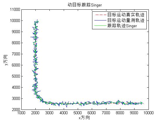
3, Operation results

4, Remarks

Version: 2014a