Implementation of linear non separable support vector machine
in the article of support vector machine, we have derived the mathematical model of linear non separable support vector machine in detail, and transformed the original problem into a dual problem to be solved. Revisit the dual problem as follows:
Final form of dual problem of linear non separable support vector machine: min α 1 2 ∑ i = 1 N ∑ j = 1 N α i α j y i y j ( x i ⋅ x j ) − ∑ i = 1 N α i s . t . ∑ i = 1 N α i y i = 0 0 ≤ α i ≤ C i = 1 , 2 , ⋯ , N \min\limits_{\alpha}\,\,\,\,\,\frac{1}{2}\sum\limits_{i=1}^N{\sum\limits_{j=1}^N{\alpha_i\alpha_jy_iy_j(x_i\cdot x_j)}}-\sum\limits_{i=1}^N{\alpha_i}\\ s.t.\,\,\,\,\,\sum\limits_{i=1}^N\alpha_i y_i=0\\ 0\le\alpha_i\le C\,\,\,\,\,i=1,2,\cdots,N αmin21i=1∑Nj=1∑Nαiαjyiyj(xi⋅xj)−i=1∑Nαis.t.i=1∑Nαiyi=00≤αi≤Ci=1,2,⋯,N
Dual problem of linear separable support vector machine:
min
α
1
2
∑
i
=
1
N
∑
j
=
1
N
α
i
α
j
y
i
y
j
(
x
i
⋅
x
j
)
−
∑
i
=
1
N
α
i
s
.
t
.
∑
i
=
1
N
α
i
y
i
=
0
α
i
≥
0
i
=
1
,
2
,
⋯
,
N
\min\limits_{\alpha}\,\,\,\,\,\frac{1}{2}\sum\limits_{i=1}^N\sum\limits_{j=1}^N{\alpha_i\alpha_jy_iy_j(x_i\cdot x_j)}-\sum\limits_{i=1}^N{\alpha_i}\\ s.t.\,\,\,\,\sum\limits_{i=1}^N{\alpha_iy_i=0}\\ \alpha_i\ge0\,\,\,\,i=1,2,\cdots,N
αmin21i=1∑Nj=1∑Nαiαjyiyj(xi⋅xj)−i=1∑Nαis.t.i=1∑Nαiyi=0αi≥0i=1,2,⋯,N
by comparing the mathematical models of the two support vector machines, it can be found that the objective functions of the two are consistent. The only difference is the constraint condition. In fact, this constraint condition only works with the support vector and has no great impact on other sample points, so we can also think that, The final learning results of linear non separable support vector machine are also only related to some sample points. We have not conducted experiments here, and the results are not known for the time being.
similarly, we use MATLAB to solve the dual problem. Similar to the linear separable implementation, we only need to change the upper bound of the independent variable, so the code is as follows:
%% The linear non separable data are classified by support vector machine, and the quadratic programming function is used to solve it
% Clear variables
clc;
clear;
% Import dataset
data = [
    27    53    -1
    49    37    -1
    56    39    -1
    28    60    -1
    68    75     1
    57    69     1
    64    62     1
    77    68     1
    70    54     1
    56    63     1
    25    41    -1
    66    34     1
    55    79     1
    77    31    -1
    46    66     1
    30    23    -1
    21    45    -1
    68    42    -1
    43    43    -1
    56    59     1
    79    68     1
    60    34    -1
    49    32    -1
    80    79     1
    77    46     1
    26    66     1
    29    29    -1
    77    34     1
    20    71    -1
    49    25    -1
    58    65     1
    33    57    -1
    31    79     1
    20    78     1
    77    37    -1
    73    34    -1
    60    26    -1
    77    66     1
    71    75     1
    35    36    -1
    49    61     1
    26    37    -1
    42    73     1
    36    50    -1
    66    73     1
    71    43     1
    33    62     1
    43    41    -1
    42    29    -1
    58    20    -1
    ];
X = data(:,1:2);
y = data(:,3);
C = 5;
% Compared with linear separable data, linear non separable data has only one more constraint in the form of quadratic programming C,So it is the same in the process of solving.
% Constructing quadratic coefficient matrix H
H = [];
for i =1:length(X)
    for j = 1:length(X)
        H(i,j) = X(i,:)*(X(j,:))'*y(i)*y(j);
    end
end
% Construct first-order term coefficient f
f = zeros(length(X),1)-1;
A = [];b = []; % Inequality constraint
Aeq = y';beq = 0; % Equality constraint
ub = ones(length(X),1).*C;lb = zeros(length(X),1); % Range of arguments
[x,fval] = quadprog(H,f,A,b,Aeq,beq,lb,ub);
% x Represents the solution of the argument, and x Function value at
% Will be very small x Direct assignment to 0
x(x < 1e-5) = 0;

% Obtained by solving x Solution coefficient w
w = [0,0];
[a,~] = find(x~=0); % Find a solution b Value of
temp = 0;
for i = 1:length(X)
    w = w + x(i)*y(i)*X(i,:);
    temp = temp + x(i)*y(i)*X(i,:)*X(a(1),:)';
end
% Calculate offset factor
b = y(a(1)) - temp;
disp(['The sample points involved are',num2str(length(a))])

% Visualization of data results
k = - w(1)/w(2); % Structural intercept type
b_ = -b/w(2); % Tectonic coefficient b
m = 0:2:90; % Generate some points
n = k*m+b_;
plot(m,n,'--black')
n_2 = k*m+b_+1/w(2);
hold on
plot(m,n_2,'--blue')
n_3 = k*m+b_-1/w(2);
plot(m,n_3,'--red');
% Classify the data into two categories to facilitate drawing
X_1 = [];
X_2 = [];
for i =1:length(y)
    if y(i)==-1
        X_1 = [X_1;X(i,:)];
    else
        X_2 = [X_2;X(i,:)];
    end
end
% HandleVisibility=off The purpose of the parameter is not to display the legend
scatter(X_1(:,1),X_1(:,2),'red','HandleVisibility','off')
hold on
scatter(X_2(:,1),X_2(:,2),'blue','HandleVisibility','off')
xlim([10,90])
grid on
title('Classification results of linear non separable support vector machine')
% Draw the position of the support vector,This is from\alpha To determine which points are support vectors.
scatter(X([14,4],1),X([14,4],2),'r','filled','HandleVisibility','off')
scatter(X(34,1),X(34,2),'b','filled','HandleVisibility','off')
% Sample points 4, 14 and 34 are points falling on the interval boundary
% Calculate relaxation variables
functiona_margin  = zeros(length(X),1);
loos = zeros(length(X),1);
for i=1:length(X)
    functiona_margin(i) = y(i)*(w*X(i,:)'+b);
    if functiona_margin(i)>1 % If the function interval meets the requirements
        loos(i) = 0; % Then this point is not a support vector point
    else
        loos(i) = 1 - functiona_margin(i); % This point is the support vector and calculates the value of the relaxation variable
    end
end
% Draw misclassification points
scatter(X([12,26,28,47],1),X([12,26,28,47],2),'*','black')

% 18 29 35 36 46 Fall between the interval boundary and the separation hyperplane
% 12,26,28,47 It belongs to misclassification point
legend('Dividing line','Category 1','Category 2','Misclassification point')
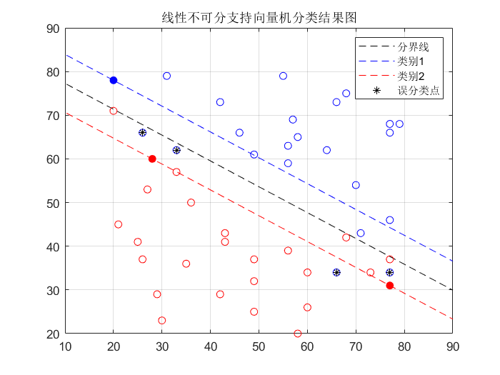
The results of the operation are as follows:

as can be seen from the above figure, the definition of support vector for linear non separable problems is much more complex than that for linear separable problems, because there are many cases of sample points at this time, including correct classification of sample points circumscribed at the interval boundary, wrong classification of sample points circumscribed at the interval boundary, wrong classification of sample points between hyperplane and interval boundary The sample points are between the hyperplane and the function boundary and the classification is correct, the sample points are on the function boundary and the classification is correct, the sample points are on the hyperplane, the sample points are on the function boundary and the classification is wrong
⋯
\cdots
* there are so many cases, of which only three cases belong to support vectors: on the function boundary, between the function boundary and the hyperplane, and on the other side of the hyperplane (when the classification is wrong). Remember that in the online separable SVM problem, support vector refers to the sample points that fall on the boundary of the function, i.e
α
i
>
0
\alpha_i>0
α i > 0, in the example where the linearity is inseparable,
α
i
>
0
\alpha_i>0
α There are many points where i > 0. We need to discuss these points.
the following discussion is based on the data in the above code. There are 50 sample points, half of which are positive and half are negative. In addition, we set the punishment intensity of relaxation variables
C
=
5
C=5
C=5 for all
α
>
0
\alpha>0
α> The sample points of 0 are discussed, and the relaxation variable size of these points is calculated. We find that:
| Support vector | α \alpha α | ξ \xi ξ | Distribution of points |
|---|---|---|---|
| 4 | 4.6812 | 0 | On interval boundary |
| 14 | 0.6572 | 0 | On interval boundary |
| 34 | 0.3384 | 0 | On interval boundary |
| 12 | 5 | 2.5292 | Misclassification point |
| 26 | 5 | 1.2738 | Misclassification point |
| 28 | 5 | 1.5477 | Misclassification point |
| 47 | 5 | 1.2523 | Misclassification point |
| 18 | 5 | 0.8554 | Between hyperplane and function interval |
| 29 | 5 | 0.9446 | Between hyperplane and function interval |
| 35 | 5 | 0.9046 | Between hyperplane and function interval |
| 36 | 5 | 0.0954 | Between hyperplane and function interval |
| 46 | 5 | 0.7262 | Between hyperplane and function interval |
except for the above 12 support vectors, there are no errors in other point classifications. The above table is the experimental result data. We can find the following rules through the observation results:
because it is specified in the optimization problem
α
\alpha
α The upper and lower bounds of
0
≤
α
≤
C
0\le\alpha\le C
0≤ α ≤ C, and here
C
C
The value of C is fixed at the beginning of the experiment. We take it as 5. In addition, we can use the formula for the relaxation variable
y
i
(
w
⋅
x
i
+
b
)
≥
1
−
ξ
i
y_i(w\cdot x_i+b)\ge1-\xi_i
yi(w⋅xi+b)≥1− ξ i) calculated. We found that:
- if α i ∗ < C , ξ i = 0 \alpha^*_i<C,\xi_i=0 α i∗<C, ξ If I = 0, the support vector x i x_i xi) just fall on the interval boundary;
- if α i ∗ = C , 0 ≤ ξ i ≤ 1 \alpha^*_i=C,0\le\xi_i\le1 α i∗=C,0≤ ξ If I ≤ 1, the classification is correct and the support vector x i x_i xi) fall between the interval boundary and the hyperplane;
- if α i ∗ = C , ξ i = 1 \alpha^*_i=C,\xi_i=1 α i∗=C, ξ If I = 1, the support vector falls on the hyperplane;
- if α i ∗ = C , ξ i > 1 \alpha^*_i=C,\xi_i>1 α i∗=C, ξ If I > 1, the support vector falls on the other side of the classification hyperplane, which belongs to misclassification point;
in fact, the above laws can be explained by the knowledge of functional interval and geometric interval, because we deduced the formula earlier
y
i
(
w
⋅
x
i
+
b
)
≥
1
y_i(w\cdot x_i+b)\ge1
yi (w ⋅ xi + b) ≥ 1, where 1 means that the functional distance from the support vector to the hyperplane is 1. When the sample point falls on the hyperplane, the formula
∣
w
x
+
b
∣
=
0
|wx+b|=0
∣ wx+b ∣ = 0 is constant, that is, if we introduce a relaxation variable
ξ
\xi
ξ Construction formula
y
i
(
w
⋅
x
i
+
b
)
≥
1
−
ξ
i
y_i(w\cdot x_i+b)\ge1-\xi_i
yi(w⋅xi+b)≥1− ξ i, when
ξ
i
\xi_i
ξ When i equals 1, it means that the sample
(
x
i
,
y
i
)
(x_i,y_i)
(xi, yi) falls on a hyperplane. This is to explain the distribution of support vectors from the perspective of function interval. As for why
α
\alpha
α Value of
C
C
C or take
<
C
<C
< C, this needs to be understood in the SMO algorithm, but here we only need to know, when
α
i
\alpha_i
α When the interval of i is greater than 0, it will have an impact on the solution of the support vector. Therefore, the number of support vectors is not only 2, but also in both soft interval and hard interval. The specific classification needs to be discussed in detail.
as mentioned earlier, penalty parameters
C
C
The function of C is to adjust the relationship between misclassification and maximum interval, when
C
C
The greater the value of C, the greater the punishment of hyperplane on misclassification points, and the algorithm should consider reducing misclassification points. When
C
C
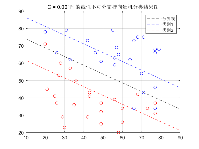
The smaller the value of C, the lower the importance of misclassification points. Refer to the following figure for details:
When set
C
C
When the value of C is 0.0001, the hyperplane is as follows:

At this time, the hyperplane will cause 5 sample points to be misclassified. Compared with
C
C
When C=5, the number of misclassification will increase by 2.