100 cases of deep learning - convolutional neural network (CNN) for license plate recognition | day 15

1, Preliminary work

My environment:

Locale: Python 3 six point five
Compiler: Jupiter notebook
Deep learning environment: tensorflow2 four point one
Data address: [portal]

Previous highlights:

100 cases of deep learning convolutional neural network (CNN) to realize mnist handwritten numeral recognition | day 1
100 cases of deep learning - convolutional neural network (CNN) color picture classification | day 2
100 cases of deep learning - convolutional neural network (CNN) garment image classification | day 3
100 cases of deep learning - convolutional neural network (CNN) flower recognition | day 4
100 cases of deep learning - convolutional neural network (CNN) weather recognition | day 5
100 cases of deep learning - convolutional neural network (VGG-16) to identify the pirate king straw hat group | day 6
100 cases of deep learning - convolutional neural network (VGG-19) to identify the characters in the spirit cage | day 7
100 cases of deep learning - convolutional neural network (ResNet-50) bird recognition | day 8
100 cases of deep learning - circular neural network (RNN) to achieve stock prediction | day 9
100 cases of deep learning - circular neural network (LSTM) to realize stock prediction | day 10
100 cases of deep learning - convolutional neural network (AlexNet) hand-in-hand teaching | day 11
Teach you how to use CNN identification verification code - 100 cases of in-depth learning | day 12
100 cases of deep learning - convolutional neural network (perception V3) recognition of sign language | day 13
This is too strong. I use it to identify traffic signs. The accuracy is as high as 97.9% | day 14

🚀 From column: 100 cases of deep learning

1. Set GPU

If the CPU is used, you can comment out this part of the code without affecting the operation.

import tensorflow as tf

gpus = tf.config.list_physical_devices("GPU")

if gpus:
    tf.config.experimental.set_memory_growth(gpus[0], True)  #Set the amount of GPU video memory and use it on demand
    tf.config.set_visible_devices([gpus[0]],"GPU")

2. Import data

import matplotlib.pyplot as plt
# Support Chinese
plt.rcParams['font.sans-serif'] = ['SimHei']  # Used to display Chinese labels normally
plt.rcParams['axes.unicode_minus'] = False  # Used to display negative signs normally

import os,PIL,random,pathlib

# Set random seeds so that the results can be reproduced as much as possible
import numpy as np
np.random.seed(1)

# Set random seeds so that the results can be reproduced as much as possible
import tensorflow as tf
tf.random.set_seed(1)

data_dir = "D:/jupyter notebook/DL-100-days/datasets/015_licence_plate"
data_dir = pathlib.Path(data_dir)

pictures_paths = list(data_dir.glob('*'))
pictures_paths = [str(path) for path in pictures_paths]
pictures_paths[:3]

['D:\\jupyter notebook\\DL-100-days\\datasets\\015_licence_plate\\000000000_hide WP66B0.jpg',
 'D:\\jupyter notebook\\DL-100-days\\datasets\\015_licence_plate\\000000001_Jin D8Z15T.jpg',
 'D:\\jupyter notebook\\DL-100-days\\datasets\\015_licence_plate\\000000002_Shaanxi Z813VB.jpg']

image_count = len(list(pictures_paths))

print("The total number of pictures is:",image_count)

Total number of pictures: 619

# Get data label
all_label_names = [path.split("_")[-1].split(".")[0] for path in pictures_paths]
all_label_names[:3]

['hide WP66B0', 'Jin D8Z15T', 'Shaanxi Z813VB']

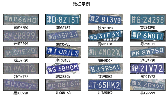
3. Data visualization

plt.figure(figsize=(10,5))
plt.suptitle("sample data",fontsize=15)

for i in range(20):
    plt.subplot(5,4,i+1)
    plt.xticks([])
    plt.yticks([])
    plt.grid(False)
    
    # display picture
    images = plt.imread(pictures_paths[i])
    plt.imshow(images)
    # Display label
    plt.xlabel(all_label_names[i],fontsize=13)

plt.show()

4. Label digitization

char_enum = ["Beijing","Shanghai","Jin","Chongqing","Hope","Jin","Meng","Liao","luck","black","Soviet","Zhejiang","Wan","Min","short name for Jiangxi province","Lu",\
              "Yu","Hubei","Hunan","Guangdong","Cinnamon","Joan","Chuan","expensive","cloud","hide","Shaanxi","Sweet","young","Rather","new","army","send"]

number   = [str(i) for i in range(0, 10)]    # Numbers from 0 to 9
alphabet = [chr(i) for i in range(65, 91)]   # Letters A to Z

char_set       = char_enum + number + alphabet
char_set_len   = len(char_set)
label_name_len = len(all_label_names[0])

# Digitize string
def text2vec(text):
    vector = np.zeros([label_name_len, char_set_len])
    for i, c in enumerate(text):
        idx = char_set.index(c)
        vector[i][idx] = 1.0
    return vector

all_labels = [text2vec(i) for i in all_label_names]

2, Build a TF data. Dataset

1. Preprocessing function

def preprocess_image(image):
    image = tf.image.decode_jpeg(image, channels=1)
    image = tf.image.resize(image, [50, 200])
    return image/255.0

def load_and_preprocess_image(path):
    image = tf.io.read_file(path)
    return preprocess_image(image)

2. Load data

Build TF data. The simplest way to use a dataset is to use from_tensor_slices method.

AUTOTUNE = tf.data.experimental.AUTOTUNE

path_ds  = tf.data.Dataset.from_tensor_slices(pictures_paths)
image_ds = path_ds.map(load_and_preprocess_image, num_parallel_calls=AUTOTUNE)
label_ds = tf.data.Dataset.from_tensor_slices(all_labels)

image_label_ds = tf.data.Dataset.zip((image_ds, label_ds))
image_label_ds

<ShuffleDataset shapes: ((50, 200, 1), (7, 69)), types: (tf.float32, tf.float64)>

train_ds = image_label_ds.take(5000).shuffle(5000)  # First 5000 batch es
val_ds   = image_label_ds.skip(5000).shuffle(1000)  # Skip the first 5000 and select the following

3. Configuration data

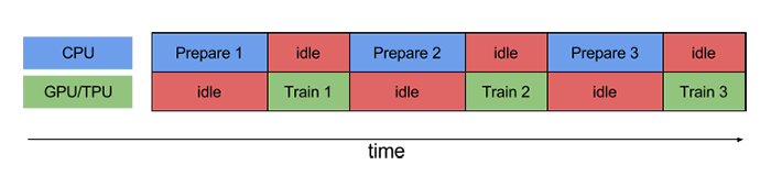
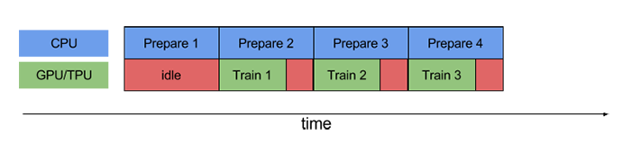
Let's review the prefetch () function first. Prefetch() function details: when the CPU is preparing data, the accelerator is idle. In contrast, when the accelerator is training the model, the CPU is idle. Therefore, the training time is the sum of CPU preprocessing time and accelerator training time. Prefetch () overlaps the preprocessing of training steps with the model execution process. When the accelerator is executing the nth training step, the CPU is preparing the data of step N+1. This can not only minimize the single step time of training (rather than the total time), but also shorten the time required to extract and transform data. If prefetch() is not used, the CPU and GPU/TPU are idle most of the time:

Using prefetch() can significantly reduce idle time:

BATCH_SIZE = 16

train_ds = train_ds.batch(BATCH_SIZE)
train_ds = train_ds.prefetch(buffer_size=AUTOTUNE)

val_ds = val_ds.batch(BATCH_SIZE)
val_ds = val_ds.prefetch(buffer_size=AUTOTUNE)
val_ds

<PrefetchDataset shapes: ((None, 50, 200, 1), (None, 7, 69)), types: (tf.float32, tf.float64)>

3, Build network model

At present, we mainly take you through the code and sort out your ideas. You can optimize the network structure and adjust the model parameters by yourself. In the future, I will also give some targeted tuning cases.

from tensorflow.keras import datasets, layers, models

model = models.Sequential([
    
    layers.Conv2D(32, (3, 3), activation='relu', input_shape=(50, 200, 1)),#Convolution layer 1, convolution kernel 3 * 3
    layers.MaxPooling2D((2, 2)),                   #Pool layer 1, 2 * 2 sampling
    layers.Conv2D(64, (3, 3), activation='relu'),  #Convolution layer 2, convolution kernel 3 * 3
    layers.MaxPooling2D((2, 2)),                   #Pool layer 2, 2 * 2 sampling
    
    layers.Flatten(),                              #Flatten layer, connecting convolution layer and full connection layer
#     layers.Dense(1000, activation='relu'),         #Full connection layer, further feature extraction
    layers.Dense(1000, activation='relu'),         #Full connection layer, further feature extraction
#     layers.Dropout(0.2),  
    layers.Dense(label_name_len * char_set_len),
    layers.Reshape([label_name_len, char_set_len]),
    layers.Softmax()                               #Output layer, output expected results
])
# Print network structure
model.summary()

Model: "sequential"
_________________________________________________________________
Layer (type)                 Output Shape              Param #   
=================================================================
conv2d (Conv2D)              (None, 48, 198, 32)       320       
_________________________________________________________________
max_pooling2d (MaxPooling2D) (None, 24, 99, 32)        0         
_________________________________________________________________
conv2d_1 (Conv2D)            (None, 22, 97, 64)        18496     
_________________________________________________________________
max_pooling2d_1 (MaxPooling2 (None, 11, 48, 64)        0         
_________________________________________________________________
flatten (Flatten)            (None, 33792)             0         
_________________________________________________________________
dense (Dense)                (None, 1000)              33793000  
_________________________________________________________________
dense_1 (Dense)              (None, 483)               483483    
_________________________________________________________________
reshape (Reshape)            (None, 7, 69)             0         
_________________________________________________________________
softmax (Softmax)            (None, 7, 69)             0         
=================================================================
Total params: 34,295,299
Trainable params: 34,295,299
Non-trainable params: 0
_________________________________________________________________

4, Set dynamic learning rate

Here are the advantages and disadvantages of high learning rate and low learning rate.

High learning rate
- Advantages: 1. Speed up the learning rate. 2. It helps to jump out of the local optimal value.
- Disadvantages: 1. Model training does not converge. 2. Only using the college attendance rate can easily lead to the inaccuracy of the model.
Low learning rate
- Advantages: 1. It is conducive to model convergence and model refinement. 2. 2. Improve model accuracy.
- Disadvantages: 1. It is difficult to jump out of the local optimal value. 2. Slow convergence.

Note: the dynamic learning rate set here is exponential decay. Before each epoch starts, the learning_rate will be reset to the initial_learning_rate, and then the attenuation will start again. The calculation formula is as follows:

learning_rate = initial_learning_rate * decay_rate ^ (step / decay_steps)

# Set initial learning rate
initial_learning_rate = 1e-3

lr_schedule = tf.keras.optimizers.schedules.ExponentialDecay(
        initial_learning_rate, 
        decay_steps=20,      # Knock on the blackboard!!! This refers to steps, not epochs
        decay_rate=0.96,     # LR will become decay after one attenuation_ rate*lr
        staircase=True)

# Feed exponential decay learning rate into optimizer
optimizer = tf.keras.optimizers.Adam(learning_rate=lr_schedule)

5, Compile

model.compile(optimizer=optimizer,
              loss='categorical_crossentropy',
              metrics=['accuracy'])

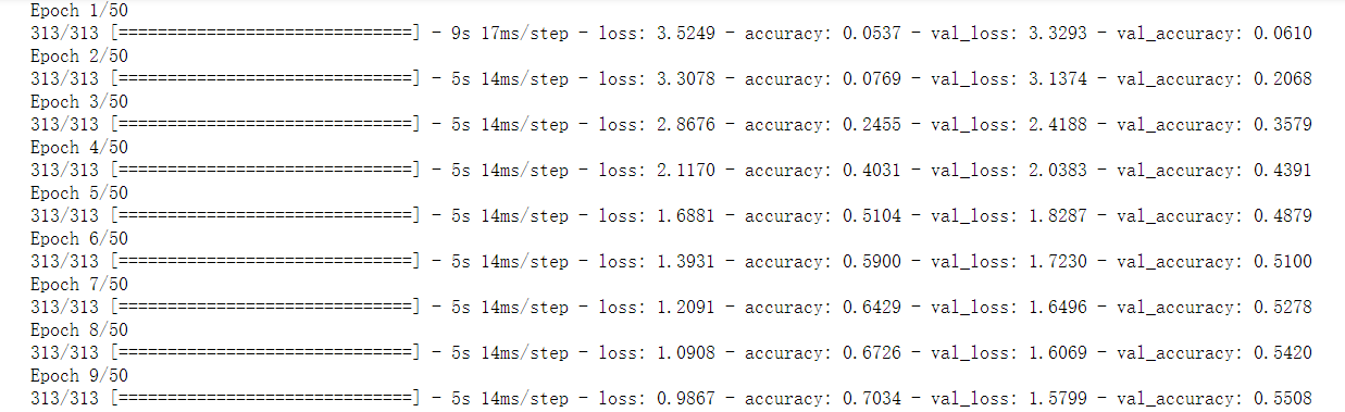
6, Training

epochs = 50

history = model.fit(
    train_ds,
    validation_data=val_ds,
    epochs=epochs
)

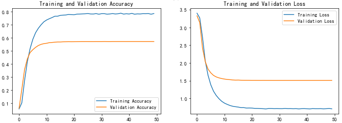
7, Model evaluation

acc = history.history['accuracy']
val_acc = history.history['val_accuracy']

loss = history.history['loss']
val_loss = history.history['val_loss']

epochs_range = range(epochs)

plt.figure(figsize=(12, 4))
plt.subplot(1, 2, 1)

plt.plot(epochs_range, acc, label='Training Accuracy')
plt.plot(epochs_range, val_acc, label='Validation Accuracy')
plt.legend(loc='lower right')
plt.title('Training and Validation Accuracy')

plt.subplot(1, 2, 2)
plt.plot(epochs_range, loss, label='Training Loss')
plt.plot(epochs_range, val_loss, label='Validation Loss')
plt.legend(loc='upper right')
plt.title('Training and Validation Loss')
plt.show()

8, Saving and loading models

# Save model
model.save('model/15_model.h5')

# Loading model
new_model = tf.keras.models.load_model('model/15_model.h5')

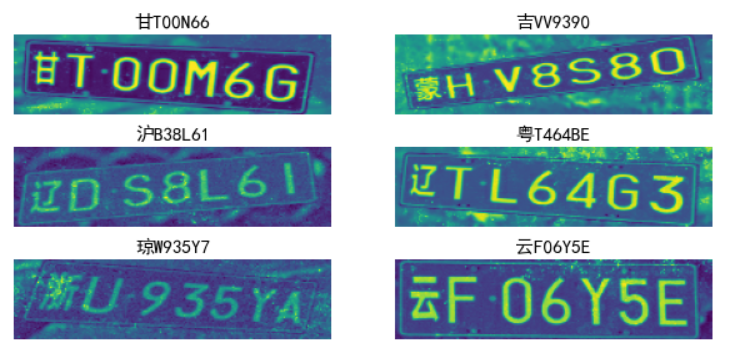
9, Forecast

def vec2text(vec):
    """
    Restore label (vector)->(string)
    """
    text = []
    for i, c in enumerate(vec):
        text.append(char_set[c])
    return "".join(text)

plt.figure(figsize=(10, 8))            # The width of the figure is 10 and the height is 8

for images, labels in val_ds.take(1):
    for i in range(6):
        ax = plt.subplot(5, 2, i + 1)  
        # display picture
        plt.imshow(images[i])

        # You need to add a dimension to the picture
        img_array = tf.expand_dims(images[i], 0) 

        # Use model prediction verification code
        predictions = model.predict(img_array)
        plt.title(vec2text(np.argmax(predictions, axis=2)[0]),fontsize=15)

        plt.axis("off")