Recently, I often hear that girls' A cup is versatile and high-grade!
Today, let's take the general sales situation of a bra brand in Jingdong Mall in different sizes to see what size is the mainstream at present!
catalogue
1. Demand sorting
2. Data acquisition
3. Statistical display
3.1. cup distribution
3.2. color distribution
4. That's it
5. Python learning resources

1. Demand sorting
Many people learn Python and don't know where to start.

Many people learn to look for python,After mastering the basic grammar, I don't know where to start.

Many people who may already know the case do not learn more advanced knowledge.

These three categories of people, I provide you with a good learning platform, free access to video tutorials, e-books, and the source code of the course!

QQ Group: 101677771

Welcome to join us and discuss and study together
This paper is relatively simple. It simply collects the commodity comments of different sizes of a bra brand with the largest number of comments from JD, and then counts the proportion of different sizes.
Since JD has no similar sales volume (or how many people pay), we only use the number of comments as the comparison dimension. We won't introduce how to obtain the number of comments here.
By selecting underwear bra suitable for young people in Jingdong, and then sorting according to the number of comments, we can get the top commodity list. Since the first two are all size-free, and the third is a bra laundry bag (also size-free), we chose the fourth product.

Looking for target brands
Then, we directly click to enter the details page of the fourth commodity and find that there are many 7 colors and 10 sizes, which is a little more.
In order to better obtain the comment data of each product, we need to obtain the product id of each product first. Therefore, we F12 entered the developer mode, searched one of the commodity IDs on the element page, and finally found the place where all the commodity IDs are stored as follows: (it can be parsed through regular analysis)
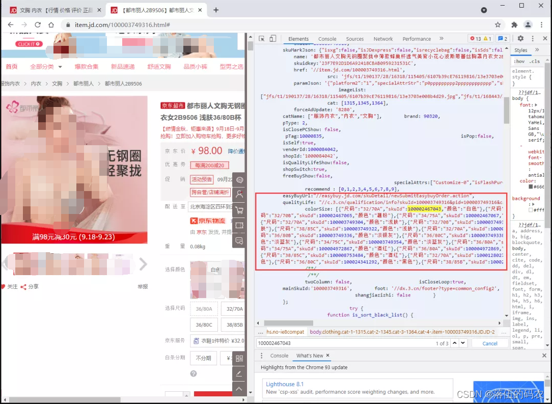
color&size
Now that you can get all the product IDS, you can call the comment interface through the product id to get the comment data of the corresponding product. Let's start coding!

2. Data acquisition
In the data collection part, first use regular to obtain all the product IDS, and then obtain the comment data corresponding to all the product IDS through the product id, then the required data will be alive.
Get all product IDS
import requests
import re
import pandas as pd
headers = {
# "Accept-Encoding": "Gzip", # Use gzip to compress and transfer data for faster access
"User-Agent": "Mozilla/5.0 (Windows NT 10.0; Win sixty-four; x sixty-four) AppleWebKit/537.36 (KHTML, like Gecko) Chrome/83.0.4103.97 Safari/537.36",
# "Cookie": cookie,
"Referer": "https://item.jd.com/"
}
url= r'https://item.jd.com/100003749316.html'
r = requests.get(url, headers=headers, timeout=6)
text = re.sub(r'\s','',r.text)
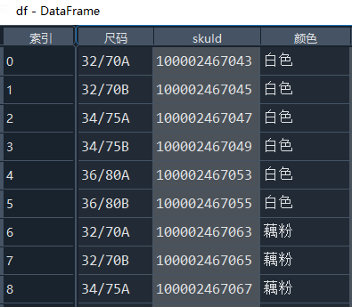
colorSize = eval(re.findall(r'colorSize:(\[.*?\])', text)[0])
df = pd.DataFrame(colorSize)
Get comment data corresponding to product id
# Get comment information
def get_comment(productId, proxies=None):
# time.sleep(0.5)
url = 'https://club.jd.com/comment/skuProductPageComments.action?'
params = {
'callback': 'fetchJSON_comment98',
'productId': productId,
'score': 0,
'sortType': 6,
'page': 0,
'pageSize': 10,
'isShadowSku': 0,
'fold': 1,
}
# print(proxies)
r = requests.get(url, headers=headers, params=params,
proxies=proxies,
timeout=6)
comment_data = re.findall(r'fetchJSON_comment98\((.*)\)', r.text)[0]
comment_data = json.loads(comment_data)
comment_summary = comment_data['productCommentSummary']
return sum([comment_summary[f'score{i}Count'] for i in range(1,6)])
df_commentCount = pd.DataFrame(columns=['skuId','commentCount'])
proxies = get_proxies()
for productId in df.skuId[44:]:
df_commentCount = df_commentCount.append({
"skuId": productId,
"commentCount": get_comment(productId, proxies),
},
ignore_index=True
)
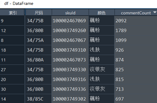
df = df.merge(df_commentCount,how='left')

3. Statistical display
Let's start with ABC in size The cup parts are listed separately
df['cup'] = df['size'].str[-1]
Let's start our simple statistical presentation
Let's first look at the overview of data information
>>> df.info()

<class 'pandas.core.frame.DataFrame'>
Int64Index: 64 entries, 0 to 63
Data columns (total 5 columns):
 #   Column        Non-Null Count  Dtype
---  ------        --------------  -----
 0   size            64 non-null     object
 1   skuId         64 non-null     object
 2   colour            64 non-null     object
 3   commentCount  64 non-null     object
 4   cup           64 non-null     object
dtypes: object(5)
memory usage: 3.0+ KB
3.1. cup distribution
However, the data we collected are only divided into three types: A-B-C cup..
cupNum = df.groupby('cup')['commentCount'].sum().to_frame('quantity')
cupNum
|
cup |
quantity |
|
A |
6049 |
|
B |
11618 |
|
C |
4076 |
import matplotlib.pyplot as plt
from matplotlib import font_manager as fm

plt.rcParams['font.sans-serif'] = ['Microsoft YaHei']
plt.rcParams['axes.unicode_minus'] = False

labels = cupNum.index
sizes = cupNum['quantity']
explode = (0, 0.1, 0)

fig1, ax1 = plt.subplots(figsize=(6,5))
patches, texts, autotexts = ax1.pie(sizes, explode=explode, labels=labels, autopct='%1.1f%%',
                                    shadow=True, startangle=90)
ax1.axis('equal')

# Reset font size
proptease = fm.FontProperties()
proptease.set_size('large')
plt.setp(autotexts, fontproperties=proptease)
plt.setp(texts, fontproperties=proptease)
ax1.set_title('cup distribution')
plt.show()

cup distribution
We can see that up to 53.4% of buyers are B-cup, followed by A-cup, accounting for 27.8%.
3.2. color distribution
colorNum = df.groupby('colour')['commentCount'].sum().to_frame('quantity')
colorNum
|
colour |
quantity |
|
Light skin |
3627 |
|
Light blue grey |
3058 |
|
Light silver grey |
3837 |
|
white |
1439 |
|
Lotus root powder |
8286 |
|
Wine red |
1429 |
|
black |
67 |
We can see that lotus root powder is the most and far ahead, followed by light silver gray, light skin and light blue.
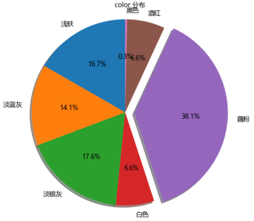
color distribution
The following are the lotus root powder colors accounting for up to 38.1%

Lotus root powder color: from Jingdong

4. That's it
We see the most 34/75B, 34 is the English code, 75 can be understood as the lower chest circumference (in fact, 34 and 75 here can be understood as the same meaning), and B is cup.
For cup and bust comparison table, refer to:
The above is all the content of this time. The sample size is small. It is not exquisite. It is only for entertainment!