1. Experimental purpose

This notebook is used for the following purposes:

• Training a single model on multiple time series
• The pre training model is used to obtain the prediction of any time series not seen during training
• Training and using models using covariates

2. Guide library

# fix python path if working locally
from utils import fix_pythonpath_if_working_locally

fix_pythonpath_if_working_locally()

import pandas as pd
import numpy as np
import torch
import matplotlib.pyplot as plt
from darts.models import NBEATSModel
from darts.models import *
from darts import TimeSeries
from darts.utils.timeseries_generation import (
    gaussian_timeseries,
    linear_timeseries,
    sine_timeseries,
)
from darts.models import (
    RNNModel,
    TCNModel,
    TransformerModel,
    NBEATSModel,
    BlockRNNModel,
)
from darts.metrics import mape, smape
from darts.dataprocessing.transformers import Scaler
from darts.utils.timeseries_generation import datetime_attribute_timeseries
from darts.datasets import AirPassengersDataset, MonthlyMilkDataset
%load_ext autoreload
%autoreload 2
%matplotlib inline

import pandas as pd
import numpy as np
import matplotlib.pyplot as plt

from darts import TimeSeries
from darts.datasets import AirPassengersDataset,MonthlyMilkDataset


# for reproducibility
torch.manual_seed(1)
np.random.seed(1)

3. Read data

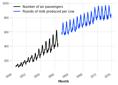
Start by reading two time series - one containing the number of airline passengers per month and the other containing the milk yield per cow per month. These time series do not have much relationship with each other, but they all have obvious annual periodicity and monthly frequency of upward trend, and (completely coincidentally) they contain values of comparable orders of magnitude.

series_air = AirPassengersDataset().load()
series_milk = MonthlyMilkDataset().load()

series_air.plot(label="Number of air passengers")
series_milk.plot(label="Pounds of milk produced per cow")
plt.legend()

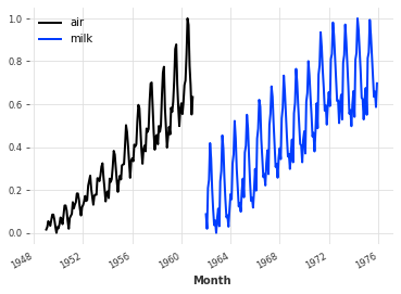
4. Pretreatment

In general, neural networks tend to work better on standardized / standardized data. Here, the Scaler class will be used to normalize the time series between 0 and 1:

from darts.dataprocessing.transformers import Scaler

scaler_air, scaler_milk = Scaler(), Scaler()
series_air_scaled = scaler_air.fit_transform(series_air)
series_milk_scaled = scaler_milk.fit_transform(series_milk)

series_air_scaled.plot(label="air")
series_milk_scaled.plot(label="milk")
plt.legend()

5. Split data set [training set, verification set]

The last 36 months of these two series are retained as validation:

train_air, val_air = series_air_scaled[:-36], series_air_scaled[-36:]
train_milk, val_milk = series_milk_scaled[:-36], series_milk_scaled[-36:]

6. Global prediction model

Darts contains many prediction models, but not all models can be trained on multiple time series. The model supporting multiple series of training is called global model. There are currently five global models:

• BlockRNN model
• RNN model
• Time convolution network (TCN)
• N-Beats model
• Transformer model

Two time series will be distinguished:

• The target time series is the time series we are interested in predicting (given its history)
• Covariate time series are time series that may help to predict the target series, but they are not interested in prediction. Sometimes referred to as external data.

Further distinguish covariate series, depending on whether they can know in advance:

• Past covariates represent time series whose past values are known at the time of prediction. These are usually things that must be measured or observed.
• Future covariates represent time series whose future values are known within the predicted time range. For example, these can represent known future holidays or weather forecasts.

Some models only use past covariates, some only use future covariates, and some models may use both.

• BlockRNNModel, TCNModel,NBEATSModel and transformer model all use past_covariates.
• RNNModel uses future_covariates.

All global models listed above support multiple sequences of training. In addition, they all support multivariable sequences. This means that they can be seamlessly used in multidimensional time series; The target series can contain one (as is often the case) or more dimensions. A time series with multiple dimensions is actually just a regular time series, in which the value of each timestamp is a vector rather than a scalar.

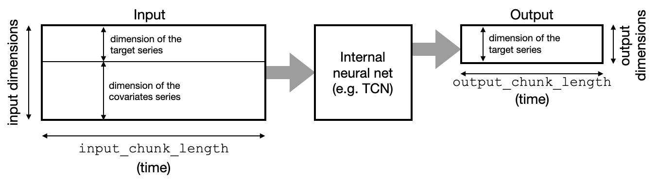
For example, past is supported_ The four models of covariables follow the "block" architecture. They contain a neural network that takes blocks of time series as input and outputs (predicted) blocks of future time series. The input dimension is the dimension (component) of the target sequence, plus the number of components of all covariates - stacked together. The output dimension is the dimension of the target sequence:

RNNModel works differently, in a circular way (which is why they support future covariates). The good news is that as users, we don't need to worry too much about different model types and input / output dimensions. Dimensions are automatically inferred by the model based on training data, and support for past or future covariates is provided by past_ Covariables or future_ The covariables parameter is handled simply.

When building the model, you still need to specify two important parameters:

• input_chunk_length: This is the length of the backtracking window of the model; Therefore, the model will read the previous input_chunk_length point to calculate each output.
• output_chunk_length: This is the length of the output (prediction) generated by the internal model. However, the predict() method of * * "outer" dart model * * (for example, NBEATSModel, TCNModel, etc.) can be called in a longer time range. In these cases, if the output is exceeded_ chunk_ If predict() is called in the range of length, the internal model will be called repeatedly, relying on its own previous output in an autoregressive manner. If past is used_ Covariables, which requires these covariates to be known long enough in advance.

7. Training prediction univariate

Build an N-BEATS model with a backtracking window of 24 points (input_chunk_length=24) and predict the next 12 points (output_chunk_length=12). Select these values so that the model will produce continuous forecasts each time over the past two years.
This model can be used like any other dart prediction model and is applicable to a single time series:

model_air = NBEATSModel(
    input_chunk_length=24, output_chunk_length=12, n_epochs=200, random_state=0
)
model_air.fit(train_air, verbose=True)

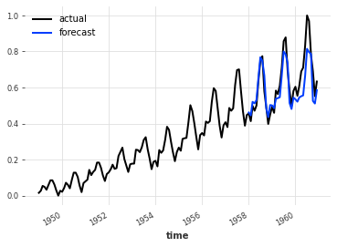
Like other dart prediction models, the prediction can be obtained by calling predict (). Note that next, the called window is 36's predict(), which is better than the internal output of the model_ chunk_ The horizon with length of 12 is longer. This is not a problem here - as explained above, in this case, the internal model will be simply called autoregressive output. In this case, it will be called three times so that the three 12 point outputs form the final 36 point prediction -- but all of this is done transparently behind the scenes.

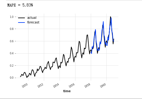
pred = model_air.predict(n=36)

series_air_scaled.plot(label="actual")
pred.plot(label="forecast")
plt.legend()
print("MAPE = {:.2f}%".format(mape(series_air_scaled, pred)))

(1). Training process [ background training process ]

Call model_ air. What happens when fit()?

To train the internal neural network, dart first creates an input / output sample data set from the provided time series (in this case, series_air_scaled). There are several ways to do this, and dart is in dart utils. The data package contains several different data set implementations.

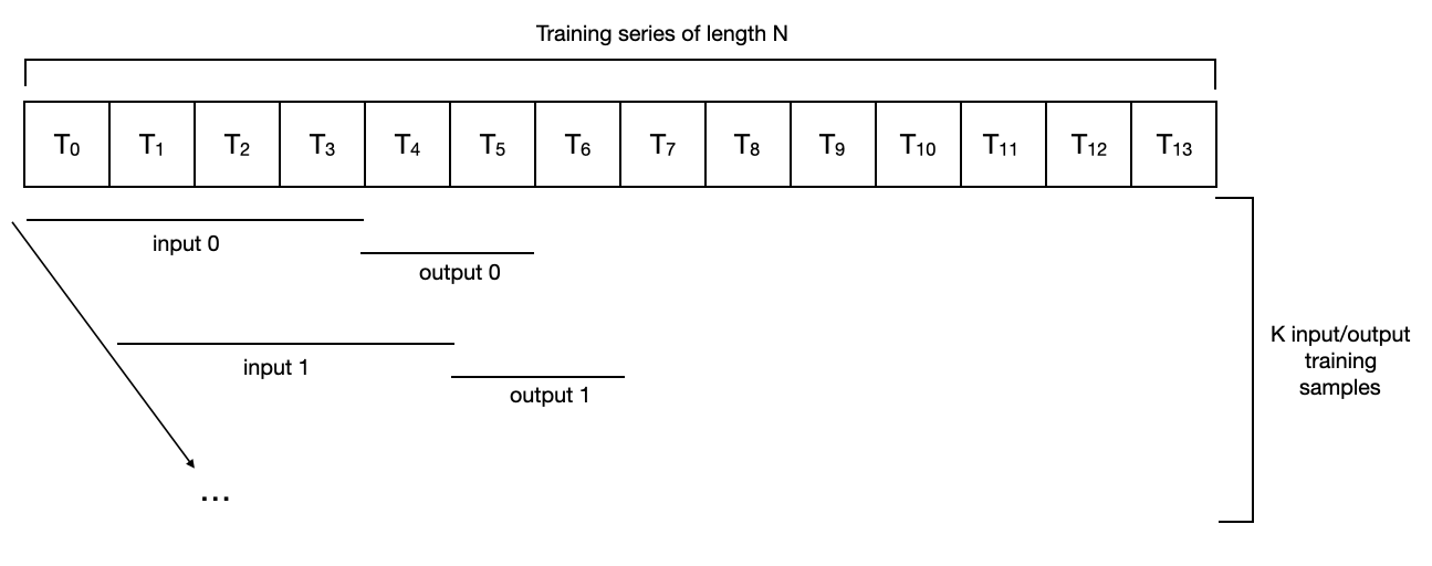
By default, NBEATSModel instantiates a darts utils. data. Pastcovariates sequentialdataset, which only constructs all continuous input / output subsequence pairs (input_chunk_length and output_chunk_length) existing in the sequence.

For a sequence of length 14, input_chunk_length=4, output_chunk_length=2, it looks like this:

For such a data set, a series of data sets with length N get N - input_ chunk_ length - output_ chunk_ Length + training set of 1 sample. In the above example, we have N=14, input_chunk_length=4 and output_chunk_length=2, so the number of samples used for training is K = 9. In this case, the training phase includes a complete traversal of all samples (possibly several small batches).

Note that by default, different models are easy to use different data sets. For example, darts utils. data. The horizonbaseddataset is inspired by the N-BEATS paper and generates samples "close to" the end of the series, and may even ignore the beginning of the series.

If you need to control how to generate training samples from instances, you can implement your own training dataset by inheriting the abstract class TimeSeries. darts. utils. data. The trainingdatasetdarts dataset inherits from the torch Dataset, which means that it is easy to implement an inert version that does not load all data into memory at once. Once you have your own dataset instance, you can call the fit directly_ from_ Dataset () method, which is supported by all global prediction models.

8. Train the model on multiple time series (multivariable)

All these machines can be used seamlessly with multiple time series. The following is a sequential data set. How to find two sequence inputs with length N and M_ chunk_ Length = 4 and output_chunk_length=2

Notes:

• Different series do not need to have the same length or even share the same timestamp.
• In fact, they don't even need to have the same frequency.
• The total number of samples in the training data set will be the union of all training samples contained in each series; So a training period will now span all samples of all series.

(1). Training air traffic data sets and milk data sequences

Another model example is fitted on two time series (air passengers and milk production). Since using two series (roughly) of the same length will double the size of the training data set, we will use half the number of epoch s:

train_air, val_air = series_air_scaled[:-36], series_air_scaled[-36:]
train_milk, val_milk = series_milk_scaled[:-36], series_milk_scaled[-36:]

model_air_milk = NBEATSModel(
    input_chunk_length=24, output_chunk_length=12, n_epochs=100, random_state=0
)

Fitting the model on two (or more) sequences is as simple as giving a list of sequences (rather than a single sequence) in the parameters of the fit() function:

model_air_milk.fit([train_air, train_milk], verbose=True)

(2). Generate prediction after training

It is important to specify the time series to predict the future when calculating the forecast: there was no such constraint before. When fitting the model on only one series, the model will remember the series internally. If predict() is called without the series parameter, it will return the (unique) prediction of the training series. Once the model applies to multiple series, this will no longer work - in this case, the series parameter becomes mandatory for predict ().

Suppose you want to predict the future of air traffic. In this example, series = train is specified for the predict() function_ Air, the purpose is to predict the train_ Contents after air:

pred = model_air_milk.predict(n=36, series=train_air)

series_air_scaled.plot(label="actual")
pred.plot(label="forecast")
plt.legend()
print("MAPE = {:.2f}%".format(mape(series_air_scaled, pred)))

(3). Does milk consumption really help predict air traffic?

In this particular example of the model, this seems to be the case (at least in terms of MAPE errors). But if you think about it, it's not surprising. Air traffic is characterized by annual seasonality and upward trend. Milk series also exhibit these two characteristics, in which case it may help the model to capture them.

Note that this points to the possibility of pre training the prediction model; Training models once and for all, and then using them to predict sequences that are not in the training set can predict the future of one variable or multiple variables. Using the model, you can really predict the future values of any other series, even those never seen during training.

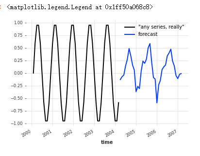
For example, suppose you want to predict the future of some arbitrary sine wave sequences: [use the trained model to predict the future of multiple variables]
This forecast is not good (sin doesn't even have the seasonality of each year), but you can understand.

any_series = sine_timeseries(length=50, freq="M")
pred = model_air_milk.predict(n=36, series=any_series)

any_series.plot(label='"any series, really"')
pred.plot(label="forecast")
plt.legend()

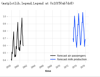
Similar to what is supported by the fit() function, you can also provide a sequence list for the predict() function in the parameter, in which case it will return a list of prediction sequences. For example, the prediction of air traffic and milk series can be obtained at one time, and these two sequences correspond to train respectively_ Air and train_ Forecast after milk:

pred_list = model_air_milk.predict(n=36, series=[train_air, train_milk])
for series, label in zip(pred_list, ["air passengers", "milk production"]):
    series.plot(label=f"forecast {label}")
plt.legend()

9. Covariate sequence

So far, the models that have been used only use the history of the target sequence to predict its future. However, as mentioned above, the global dart model also supports the use of covariate time series. These are time series of "external data", which may not be interested in prediction, but they still want to be used as inputs to the model, because they may contain valuable information.

(1) Construct covariates

Look at a simple example of air and milk series. In this example, we will try to use year and month as covariates:

# Build year and month series:
air_year = datetime_attribute_timeseries(series_air_scaled, attribute="year")
air_month = datetime_attribute_timeseries(series_air_scaled, attribute="month")

milk_year = datetime_attribute_timeseries(series_milk_scaled, attribute="year")
milk_month = datetime_attribute_timeseries(series_milk_scaled, attribute="month")

# Stack the year and month to get a two-dimensional (year and month) sequence:
air_covariates = air_year.stack(air_month)
milk_covariates = milk_year.stack(milk_month)

# Zoom between 0 and 1:
scaler_dt_air = Scaler()
air_covariates = scaler_dt_air.fit_transform(air_covariates)

scaler_dt_milk = Scaler()
milk_covariates = scaler_dt_milk.fit_transform(milk_covariates)

# Split training / validation set:
air_train_covariates, air_val_covariates = air_covariates[:-36], air_covariates[-36:]
milk_train_covariates, milk_val_covariates = (
    milk_covariates[:-36],
    milk_covariates[-36:],
)

# Draw covariates:
plt.figure()
air_covariates.plot()
plt.title("Air traffic covariates (year and month)")

plt.figure()
milk_covariates.plot()
plt.title("Milk production covariates (year and month)")

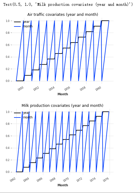
Good, so for each target sequence (air and milk), we have constructed a covariate series with the same timeline and containing years and months.

Note that the covariate series here are multivariate time series: they contain two dimensions - one represents the year and the other represents the month.

(2) Training [covariant + characteristics, target data]

Build a blockrnmodel training:

model_cov = BlockRNNModel(
    model="LSTM",
    input_chunk_length=24,
    output_chunk_length=12,
    n_epochs=300,
    random_state=0,
)

Now, to train the model with covariates, just take covariates (in the form of a list matching the target sequence) as the future_ Provide the covariables parameter to the fit() function. The parameter name is future_ Covariables to remind the model that the future values of these covariates can be used for prediction.

model_cov.fit(
    series=[train_air, train_milk],
    past_covariates=[air_train_covariates, milk_train_covariates],
    verbose=True,
)

(3) Use covariates to predict the future [no need to enter the real value of the future]

Similarly, to get the forecast, you now only need to specify the future for the predict() function_ Covariables parameter.

pred_cov = model_cov.predict(n=36, series=train_air, past_covariates=air_covariates)

series_air_scaled.plot(label="actual")
pred_cov.plot(label="forecast")
plt.legend()

Note that predict() is called here, and its prediction range n is greater than the output used in the training model_ chunk_ length. This can be achieved because even if BlockRNNModel uses past covariates, in this case, these covariates also know the future. Therefore, dart can calculate and predict the future n time steps by autoregression.

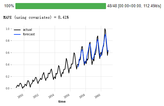
(4) Backtesting using covariates

Covariates can be used to back test the model. For example, to evaluate the 12-month operating accuracy, start with 75% of the air series:

backtest_cov = model_cov.historical_forecasts(
    series_air_scaled,
    past_covariates=air_covariates,
    start=0.6,
    forecast_horizon=12,
    stride=1,
    retrain=False,
    verbose=True,
)

series_air_scaled.plot(label="actual")
backtest_cov.plot(label="forecast")
plt.legend()
print("MAPE (using covariates) = {:.2f}%".format(mape(series_air_scaled, backtest_cov)))