preface

In the previous blog post, we learned Dimension reduction algorithm PCA , and Parameters of PCA . This article is based on the premise of having a certain foundation for PCA. This paper mainly introduces the application of PCA algorithm in practice. Including the selection of PCA parameters, the use of PCA in training set and test set, so as to solve the confusion in the practical application of PCA. This article uses Digital recognizer dataset on kaggle.

Topic

Programming environment

• python3.7
• anaconda
• jupyter notebook

Data preparation

Can pass Official channels Data can also be obtained through Data uploaded by bloggers Download.
The dataset used this time is kaggle's digital recognizer dataset. The dataset contains three csv files, as shown in the following figure

sample_submission.csv is the csv file format submitted to kaggle. train.csv is a training set of data, including 784 features and a label column. A total of 42000 sets of data. test.csv is a test set, which contains 784 features. There is no label column in this data set, with a total of 28000 groups of data. Only the training set in this dataset is used this time. The original training set is divided into new training set and test set by sklearn.

Guide Package

import pandas as pd
import numpy as np
import matplotlib.pyplot as plt
from sklearn.decomposition import PCA # PCA dimensionality reduction algorithm
from sklearn.ensemble import RandomForestClassifier
from sklearn.model_selection import cross_val_score # Cross test
from sklearn.neighbors import KNeighborsClassifier # KNN classifier
from sklearn.model_selection import train_test_split # Split training set

%matplotlib inline

Import data

file = "../data/digit-recognizer/train.csv" # Change to your own local dataset path

df = pd.read_csv(file)

df.shape #(42000, 785)
# It can be seen that the data set is very large

# Feature label separation
X = df.loc[:, df.columns != 'label']
y = df.loc[:, df.columns == 'label'].values.ravel()

Selection of PCA parameters

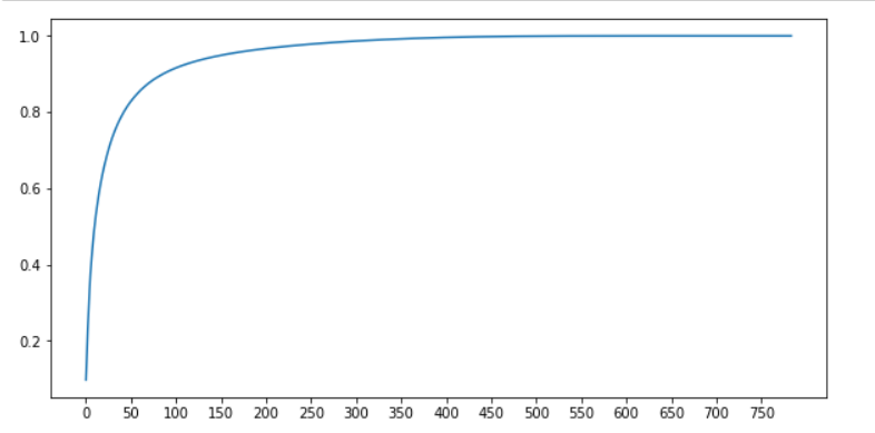
Draw the cumulative sum curve of feature information after dimension reduction

In this step, PCA does not set any parameters artificially, and uses the default value of PCA. Through explained_variance_ratio_ The proportion of the information amount of the new feature obtained by the attribute to the information amount of the original information

# The default return value PCA returns the number of features as min(shape(X))
# Obtain the amount of information of the feature after one change
pca_default = PCA()
X_defaule = pca_default.fit_transform(X)

# Proportion of information obtained for each new feature
explained_vars = pca_default.explained_variance_ratio_

# Pass NP Cumsum calculates the cumulative sum of feature information
var_sum = np.cumsum(explained_vars)

# Draw the cumulative sum curve of feature information
plt.figure(figsize=(10, 5))
plt.plot(range(X.shape[1]), var_sum)
plt.xticks(range(0, X.shape[1], 50))
plt.show()

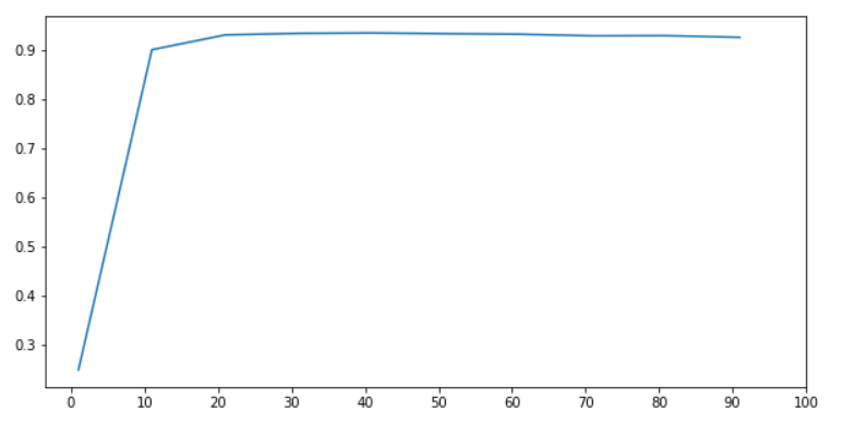
Combined with the model, n is further selected_ Value of components

As mentioned earlier, right n_ The components parameter is generally selected at the turning point of the curve.

# For n_ The selection of components generally selects the value near the turning point on the curve
# It can be seen from the figure that the turning point is between 50-100
# At 50, the amount of information has reached 80%, and at 100, the amount of information has reached nearly 90%
# Continue online, the amount of information increases slowly. Continue to struggle with more features
# It is contrary to our purpose of dimensionality reduction. The index selects 0-100 with smaller features
# We can know that there must be a value between 0 and 100 that we need
# Next, n_ The components are set between 0-100 and are scored by the model
# Select the better parameters

n_components = range(1, 101, 10)
scores = []
for i in n_components :
    X_new = PCA(n_components=i).fit_transform(X)
    scores.append(cross_val_score(RandomForestClassifier(n_estimators=21, random_state=1),
                                 X_new, y, cv=5).mean())

fig = plt.figure(figsize=(10, 5))
plt.plot(n_components, scores)
plt.xticks(range(0, 101, 10))
plt.show()

Combined with the model, the best parameters are found

# As can be seen from the figure, our model can perform well with only 10 features
# When the number of features is 20, the performance of the model is the best, which is a learning curve with a step size of 10
# The following is a detailed learning curve
# Control the number of features between 10-30, draw a learning curve and determine the final PCA parameters
n_components = range(10, 30)
scores = []
for i in n_components :
    X_new = PCA(n_components=i).fit_transform(X)
    scores.append(cross_val_score(RandomForestClassifier(n_estimators=21, random_state=1),
                                 X_new, y, cv=5).mean())

fig = plt.figure(figsize=(10, 5))
plt.plot(n_components, scores)
plt.xticks(range(9, 31))
plt.show()

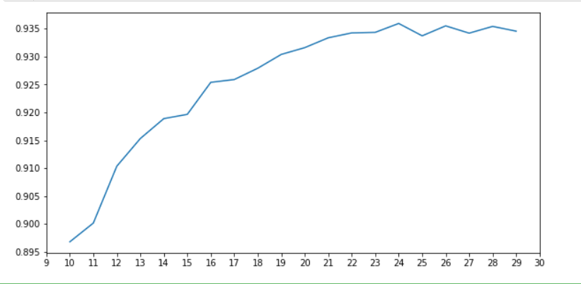
As can be seen from the figure, when n_ When components = 24, the table selection of the model is the best
After determining the best parameters of PCA, we need to adjust the parameters of the model in order to push the performance of the model to the best. about Parameter adjustment of random forest Look at my previous blog. The parameter adjustment is not shown here. If the performance of the model has not been greatly improved after adjusting parameters, you can consider changing a model. However, the problems that may be encountered in changing the model are: PCA dimensionality reduction may need to be carried out again.

KNN model performance

# After PCA dimensionality reduction, there are only 24 features, compared with the previous 784 features
# There is no doubt that there is a lot less. Here you can choose to use KNN model to try
X_final = PCA(n_components=24).fit_transform(X)
knn = KNeighborsClassifier()
score = cross_val_score(knn, X_final, y, cv=10).mean()
print(score) # 0.971355806769633

PCA is used for training set and test set

The parameters of PCA have been selected above. But there is still a doubt for us. That is how to make my dimensionality reduction PCA applicable to training set and test set. Here, the above data will be used for explanation.

Two possible ideas

• Idea 1: directly instantiate PCA and retrain sister respectively, and fit on the test set_ Transform to get new features
• Idea 2: instantiate PCA, conduct PCA training on the training set, and apply the trained PCA to the training set and the test set.
  Obviously, the second idea is correct. This idea can refer to the process of model training application.

Comparison of two ideas

Division of training set and test set

X_train, X_test, y_train, y_test = train_test_split(X, y, test_size=0.3, random_state=3)

Idea I result

# pca is used on the test set instead of fit direct retraining set
# *******************************
pca_24 = PCA(n_components=24)
# ********************************
pca_X_train = pca_24.fit_transform(X_train)
pca_X_test = pca_24.fit_transform(X_test)
knn = KNeighborsClassifier()
knn.fit(pca_X_train, y_train)
score = knn.score(pca_X_test, y_test)
print(score) # 0.7936507936507936
# It's hard to imagine that it has 79% accuracy. This is a very good shipment
# The previous performance was only about 0.3. It shows that the division of training set and test set is very perfect

Train of thought II results

# pca after fit
# pca is used on the test set instead of fit direct retraining set
# ******************************************
pca_24 = PCA(n_components=24).fit(X_train)
# *******************************************
pca_X_train = pca_24.transform(X_train)
pca_X_test = pca_24.transform(X_test)
knn = KNeighborsClassifier()
knn.fit(pca_X_train, y_train)
score = knn.score(pca_X_test, y_test)
print(score) # 0.9691269841269842

Comparing the two results, it can be seen that it is obviously the right way to apply pca after training. The performance of the model is a qualitative leap.

summary

Here, the basics of PCA have been learned. It should be noted that the selection method of PCA parameters. The use of PCA retraining set and test set must be "trained". The use of PCA retraining set and test set must be "trained". The use of PCA retraining set and test set must be "trained".. Important things are to be repeated for 3 times.

Welcome to discuss with me in the comment area and learn from each other