↑ ↑ ↑ follow the "Star" Datawhale
Daily dry goods& Team learning every month
, don't miss it
Datawhale dry
Author: Chen Kai, member of Datawhale, Sun Yat sen University
Recently, many readers have left messages, hoping to have a complete data analysis project to practice. I have collected the recommendations of the organization members these days. As the most classic enlightenment data analysis project, Titanic survival prediction should be the most appropriate for beginners. More advanced data analysis projects will be shared later. If you already have a foundation, recommend:
1. Open source project "hands on data analysis":
https://github.com/datawhalechina/hands-on-data-analysis
- DCIC 2020 algorithm analysis competition : DCIC is a rare classic event in China to open real government data, which provides a good opportunity for capacity practice and academic research.
https://mp.weixin.qq.com/s/-fzQIlZRig0hqSm7GeI_Bw
The full text is as follows:
Combined with the survival prediction of Titanic, this paper starts from 1 Data exploration (data visualization), 2 Data preprocessing, 3 Model training, 4 The four steps of model parameter adjustment are completely sorted out:

1. Data overview and visualization
1.1 data overview
First, we import our training data and test data:
The dataset contains train CSV and test CSV two files, in the Datawhale public number reply data set, can get the package link, or can be downloaded directly on the official account of kaggle.
    train_data = pd.read_csv("input/train.csv", index_col=0)
    test_data = pd.read_csv("input/test.csv", index_col=0)
    train_data.head()

train_data.describe()
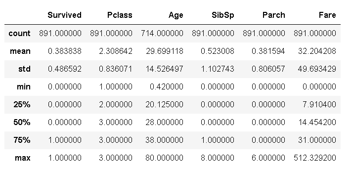
Through the describe() function, we can simply see which are numeric data and which are character data. Of course, character data should be converted into numeric data for processing, such as 0-1 encoded numeric data, but it should be noted that some numeric data may not need further processing, such as the Pclass feature, From the name, we can see that this is the characteristic of identifying the bin level. The value range is [1],
2, 3], this feature should not be simply regarded as a numerical data into the classification model and run directly, but should be transformed into one-
hot coding to identify different positions of passengers. This step will be completed in the data preprocessing step.
Let's look at the data with null value. This is what we need to further deal with later:
train_data.isnull().sum().sort_values(ascending=False).head(4)
The display result is:
>     Cabin       687
>     Age         177
>     Embarked      2
>     Fare          0
>     dtype: int64
>
[/code]

##  1.2 data visualization

In order to make this article look a little more (wrong), we can draw multi-point diagrams to show the data information. Readers who want to directly preprocess the data can skip this part, which is mostly from Kaggle An article on the official website notebook.

###  1.2.1 gender and survival

First of all, we should remember the touching "women first" strategy in the film:

```code
    sns.barplot(x="Sex", y="Survived", data=train_data)
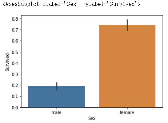 here we can see that the survival rate of women is much higher than that of men, which is also in line with the plot of the film.
1.2.2 position level (social level) and survival rate
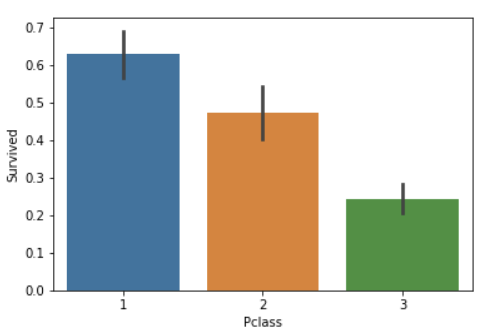
We can also guess that passengers in different positions should have different rescue rates:
    #draw a bar plot of survival by Pclass
    sns.barplot(x="Pclass", y="Survived", data=train)

    #print percentage of people by Pclass that survived
    print("Percentage of Pclass = 1 who survived:", train["Survived"][train["Pclass"] == 1].value_counts(normalize = True)[1]*100)

    print("Percentage of Pclass = 2 who survived:", train["Survived"][train["Pclass"] == 2].value_counts(normalize = True)[1]*100)

    print("Percentage of Pclass = 3 who survived:", train["Survived"][train["Pclass"] == 3].value_counts(normalize = True)[1]*100)
    Percentage of Pclass = 1 who survived: 62.96296296296296
    Percentage of Pclass = 2 who survived: 47.28260869565217
    Percentage of Pclass = 3 who survived: 24.236252545824847
The data result is still very realistic. Your position naturally has a higher survival rate. Otherwise, why do I spend this unjust money? Everyone is not equal in front of life and death.
As predicted, people with higher socioeconomic class had a higher rate of
survival. (62.9% vs. 47.3% vs. 24.2%)
1.2.3 number of family members and survival rate
    #draw a bar plot for SibSp vs. survival
    sns.barplot(x="SibSp", y="Survived", data=train)

    #I won't be printing individual percent values for all of these.
    print("Percentage of SibSp = 0 who survived:", train["Survived"][train["SibSp"] == 0].value_counts(normalize = True)[1]*100)

    print("Percentage of SibSp = 1 who survived:", train["Survived"][train["SibSp"] == 1].value_counts(normalize = True)[1]*100)

    print("Percentage of SibSp = 2 who survived:", train["Survived"][train["SibSp"] == 2].value_counts(normalize = True)[1]*100)
    Percentage of SibSp = 0 who survived: 34.53947368421053
    Percentage of SibSp = 1 who survived: 53.588516746411486
    Percentage of SibSp = 2 who survived: 46.42857142857143
 it can be seen here that those with one brother and sister generally have a higher survival rate, so go and encourage parents to have a brother and sister~
In general, it's clear that people with more siblings or spouses aboard were
less likely to survive. However, contrary to expectations, people with no
siblings or spouses were less to likely to survive than those with one or
two. (34.5% vs 53.4% vs. 46.4%)
    #draw a bar plot for Parch vs. survival
    sns.barplot(x="Parch", y="Survived", data=train)
    plt.show()
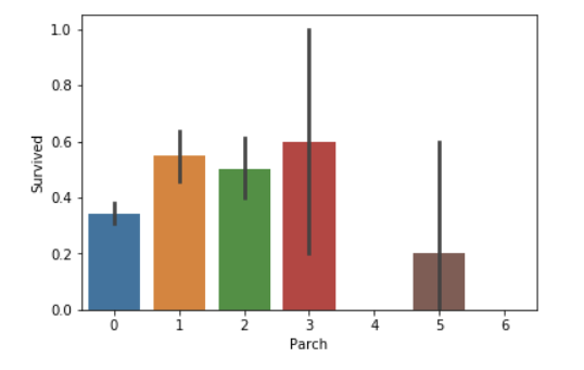 it seems that people who travel alone have a lower survival rate. Think of the wet eyes
People with less than four parents or children aboard are more likely to
survive than those with four or more. Again, people traveling alone are less
likely to survive than those with 1-3 parents or children.
1.2.4 age and survival
    #sort the ages into logical categories
    train["Age"] = train["Age"].fillna(-0.5)
    test["Age"] = test["Age"].fillna(-0.5)
    bins = [-1, 0, 5, 12, 18, 24, 35, 60, np.inf]
    labels = ['Unknown', 'Baby', 'Child', 'Teenager', 'Student', 'Young Adult', 'Adult', 'Senior']
    train['AgeGroup'] = pd.cut(train["Age"], bins, labels = labels)
    test['AgeGroup'] = pd.cut(test["Age"], bins, labels = labels)

    #draw a bar plot of Age vs. survival
    sns.barplot(x="AgeGroup", y="Survived", data=train)
    plt.show()
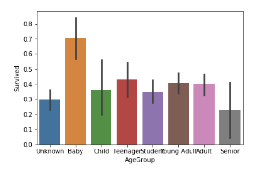
This chart is drawn using a method of pandas: cut (), which can be used to segment the data. We have an obvious conclusion that the survival rate of infants is God damn high (I think a large part of the reason is that they don't occupy space)
1.2.5 existence of position characteristics and survival rate
This is a strange indicator. According to the author:
I think the idea here is that people with recorded cabin numbers are of
higher socioeconomic class, and thus more likely to survive.
Well, let's see:
    test["CabinBool"] = (test["Cabin"].notnull().astype('int'))

    #calculate percentages of CabinBool vs. survived
    print("Percentage of CabinBool = 1 who survived:", train["Survived"][train["CabinBool"] == 1].value_counts(normalize = True)[1]*100)

    print("Percentage of CabinBool = 0 who survived:", train["Survived"][train["CabinBool"] == 0].value_counts(normalize = True)[1]*100)
    #draw a bar plot of CabinBool vs. survival
    sns.barplot(x="CabinBool", y="Survived", data=train)
    plt.show()
> Percentage of CabinBool = 1 who survived: 66.66666666666666
> Percentage of CabinBool = 0 who survived: 29.985443959243085
>
[/code]
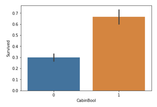
The brain hole is really big, and the result is really good~
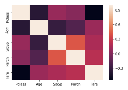
### 1.2.6 thermodynamic diagram
We can also draw a beautiful thermal map for the data, although it is of little use:
# 2. Data preprocessing
## 2.1 splice dataset
First, let's talk about the focus of training Survived Feature extraction is the objective function we need to predict, and so is this part train_data and test_data Next, we can talk about the data of the training set and the test set to be spliced together for data preprocessing. Of course, we can't know the test data in practice, but we can handle it uniformly for convenience in the competition:
```code
y_train = train_data.pop("Survived")
data_all = pd.concat((train_data, test_data), axis=0)
2.2 process the Name feature and extract the Title
Looking from left to right, we can first see that the feature Name is more eye-catching. Many people may directly remove it, but careful observation shows that this column of features contains the prefix of the Name, such as "Mr.", ”Mrs. "," Miss ", etc. as long as you have studied English in grade one of primary school, you know that this feature will represent class status and marriage to a certain extent. We can map this feature as follows:
    title = pd.DataFrame()
    title["Title"] = data_all["Name"].map(lambda name:name.split(",")[1].split(".")[0].strip())
    # title.head()
    Title_Dictionary = {
        "Capt":       "Officer",
        "Col":        "Officer",
        "Major":      "Officer",
        "Jonkheer":   "Royalty",
        "Don":        "Royalty",
        "Sir" :       "Royalty",
        "Dr":         "Officer",
        "Rev":        "Officer",
        "the Countess":"Royalty",
        "Dona":       "Royalty",
        "Mme":        "Mrs",
        "Mlle":       "Miss",
        "Ms":         "Mrs",
        "Mr" :        "Mr",
        "Mrs" :       "Mrs",
        "Miss" :      "Miss",
        "Master" :    "Master",
        "Lady" :      "Royalty"
    }
    title[ 'Title' ] = title.Title.map(Title_Dictionary)
    title = pd.get_dummies(title.Title)
    # title.head()
    data_all = pd.concat((data_all, title), axis=1)
    data_all.pop("Name")
    data_all.head()
What does the above paragraph mean? We can classify many kinds of title features first, such as "Don", "Sir" and "Jonkheer". The occurrence times of these titles are very low, about less than ten per title. Therefore, we can classify those with similar meaning into one category for the convenience of model operation. Then we use get_dummies to convert these features into one-
hot vector, the results are as follows:

2.3 extracting other features
this
The Ticket feature is troublesome and lazy. Delete it first, and then the bin feature should be very useful. Think about it, of course, the distance from our different positions on the ship to the safe passage will vary with the bin position. We simply extract the positions A, B, C and D as features, regardless of the numbers in C85 and C123 (indicating the position in A warehouse), Of course, since some ships may have safe channels in positions A, B, C and D, it may be more suitable for us to extract the following figures. For convenience, we won't discuss this first:
    data_all["Cabin"].fillna("NA", inplace=True)
    data_all["Cabin"] = data_all["Cabin"].map(lambda s:s[0])
    data_all.pop("Ticket")
As mentioned earlier, Pclass is more suitable to appear as one hot feature. We first convert it into character feature and then classify it. Here, we conveniently make several reliable category labels as one hot feature:
    data_all["Pclass"] = data_all["Pclass"].astype(str)
    feature_dummies = pd.get_dummies(data_all[["Pclass", "Sex", "Embarked", "Cabin"]])
    # feature_dummies.head()
    data_all.drop(["Pclass", "Sex", "Embarked", "Cabin"], inplace=True, axis=1)
    data_all = pd.concat((data_all, feature_dummies), axis=1)
    data_all.head()
So we expanded the feature set from the original 11 columns to 27 columns. Oh, no, we forgot to fill in the missing values. It's not too late to do it now:
    mean_cols = data_all.mean()
    data_all = data_all.fillna(mean_cols)
Here, the average value is used to fill in the two features of Age and embanked. Because Age is just a numerical feature, this filling method is reasonable, and embanked has only two missing values, so filling it casually ~ doesn't matter.
2.4 re separate the training set and the test set
Before building the model, don't forget the training set and test set we put together. Oh, remember the index when we first read the data_ Col, it comes in handy here:
    train_df = data_all.loc[train_data.index]
    test_df = data_all.loc[test_data.index]
    print(train_df.shape, test_df.shape)
The print result is (891, 27) (418, 27), which is consistent with the size of the original training set and test set. This is the end of our rough data preprocessing. Let's build the model ~
3. Model training
3.1 Random Forest
First, import the package of sklearn
    from sklearn.ensemble import RandomForestClassifier
    from sklearn.model_selection import cross_val_score
    import sklearn
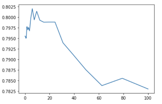
Then set different maximum tree depths for parameter tuning:
    %matplotlib inline
    depth_ = [1, 2, 3, 4, 5, 6, 7, 8]
    scores = []
    for depth in depth_:
        clf = RandomForestClassifier(n_estimators=100, max_depth=depth, random_state=0)
        test_score = cross_val_score(clf, train_df, y_train, cv=10, scoring="precision")
        scores.append(np.mean(test_score))
    plt.plot(depth_, scores)

We have obtained such a graph, which roughly reflects the maximum depth of the tree in the model, with 6 as the best. At this time, the verification accuracy can reach about 0.84. Of course, we can continue to adjust other parameters to obtain better results, but next, we will continue to discuss other models.
3.2 Gradient Boosting Classifier
The code is similar to the above:
    from sklearn.ensemble import GradientBoostingClassifier
    depth_ = [1, 2, 3, 4, 5, 6, 7, 8]
    scores = []
    for depth in depth_:
        clf = GradientBoostingClassifier(n_estimators=100, max_depth=depth, random_state=0)
        test_score = cross_val_score(clf, train_df, y_train, cv=10, scoring="precision")
        scores.append(np.mean(test_score))
    plt.plot(depth_, scores)
 has the highest success rate, which seems to be close to 0.82
3.3 Bagging
Bagging puts a lot of small classifiers together, each train a random part of the data, and then combines their final results (majority voting system)
    from sklearn.ensemble import BaggingClassifier
    params = [1, 10, 15, 20, 25, 30, 40]
    test_scores = []

    for param in params:
        clf = BaggingClassifier(n_estimators=param)
        test_score = cross_val_score(clf, train_df, y_train, cv=10, scoring="precision")
        test_scores.append(np.mean(test_score))
    plt.plot(params, test_scores)
The results are unstable and bad:

3.4 RidgeClassifier
Let's stop talking nonsense and try one by one:
    from sklearn.linear_model import RidgeClassifier
    alphas = np.logspace(-3, 2, 50)
    test_scores = []

    for alpha in alphas:
        clf = RidgeClassifier(alpha)
        test_score = cross_val_score(clf, train_df, y_train, cv=10, scoring="precision")
        test_scores.append(np.mean(test_score))
    plt.plot(alphas, test_scores)
3.5 RidgeClassifier + Bagging
    ridge = RidgeClassifier(alpha=5)
    params = [1, 10, 15, 20, 25, 30, 40]
    test_scores = []

    for param in params:
        clf = BaggingClassifier(n_estimators=param, base_estimator=ridge)
        test_score = cross_val_score(clf, train_df, y_train, cv=10, scoring="precision")
        test_scores.append(np.mean(test_score))
    plt.plot(params, test_scores)

The result is slightly better than the Bagging strategy using the default model.
3.6 XGBClassifier
    from xgboost import XGBClassifier
    params = [1, 2, 3, 4, 5, 6]
    test_scores = []
    for param in params:
        clf = XGBClassifier(max_depth=param)
        test_score = cross_val_score(clf, train_df, y_train, cv=10, scoring="precision")
        test_scores.append(np.mean(test_score))
    plt.plot(params, test_scores)

3.7 neural network
Firstly, we built a simple neural network architecture based on Keras:
    import tensorflow as tf
    import keras
    from keras.models import Sequential
    from keras.layers import *

    tf.keras.optimizers.Adam(
        learning_rate=0.003, beta_1=0.9, beta_2=0.999, epsilon=1e-07, amsgrad=False,
        name='Adam',
    )
    model = Sequential()
    model.add(Dense(32, input_dim=train_df.shape[1],kernel_initializer = 'uniform', activation='relu'))
    model.add(Dense(32, kernel_initializer = 'uniform', activation = 'relu'))
    model.add(Dropout(0.4))
    model.add(Dense(32,kernel_initializer = 'uniform', activation = 'relu'))
    model.add(Dense(1, activation='sigmoid'))

    model.compile(loss='binary_crossentropy', optimizer='adam', metrics=['accuracy'])
Then put the model into the train_df training results:
history = model.fit(np.array(train_df), np.array(y_train), epochs=20, batch_size=50, validation_split = 0.2)
The results of the last round are:
    Epoch 20/20
    712/712 [==============================] - 0s 43us/step - loss: 0.4831 - accuracy: 0.7978 - val_loss: 0.3633 - val_accuracy: 0.8715
We can see that the experimental results are still good. Let's take a look at the model architecture:
model.summary()
    Model: "sequential_1"
    _________________________________________________________________
    Layer (type)                 Output Shape              Param #
    =================================================================
    dense_1 (Dense)              (None, 32)                896
    _________________________________________________________________
    dense_2 (Dense)              (None, 32)                1056
    _________________________________________________________________
    dropout_1 (Dropout)          (None, 32)                0
    _________________________________________________________________
    dense_3 (Dense)              (None, 32)                1056
    _________________________________________________________________
    dense_4 (Dense)              (None, 1)                 33
    =================================================================
    Total params: 3,041
    Trainable params: 3,041
    Non-trainable params: 0
    _________________________________________________________________
Test model:
    scores = model.evaluate(train_df, y_train, batch_size=32)
    print(scores)
    891/891 [==============================] - 0s 18us/step
    [0.4208374666645872, 0.8316498398780823]
You can see that the effect is similar to the best effect of random forest.
4. Model optimization (parameter adjustment)
Later, we can get better scores through the second level learning of these better models.
First, we put some good results obtained before (only one parameter is adjusted here):
    from sklearn.ensemble import RandomForestClassifier, GradientBoostingClassifier, BaggingClassifier, AdaBoostClassifier
    from xgboost import XGBClassifier
    from sklearn.model_selection import cross_val_score
    from sklearn.linear_model import RidgeClassifier
    import sklearn

    classifier_num = 5
    clf = [0 for i in range(classifier_num)]
    clf[0] = RandomForestClassifier(n_estimators=100, max_depth=6, random_state=0)
    clf[1] = GradientBoostingClassifier(n_estimators=100, max_depth=4, random_state=0)
    clf[2] = RidgeClassifier(5)
    clf[3] = BaggingClassifier(n_estimators=15, base_estimator=clf[2])
    clf[4] = XGBClassifier(max_depth=2)

    from sklearn.model_selection import train_test_split
    X_train, X_test, Y_train, Y_test = train_test_split(train_df, y_train, random_state=0)

    predictFrame = pd.DataFrame()
    for model in clf:
        model.fit(X_train, Y_train)
        predictFrame[str(model)[:13]] = model.predict(X_test)
    predictFrame.head()

The name is optional. Anyway, as long as it is not repeated ~ then put this result into the next classifier for learning. I didn't try anything else, but directly put it into the random forest classifier:
    %matplotlib inline
    depth_ = [1, 2, 3, 4, 5, 6, 7, 8]
    scores = []
    for depth in depth_:
        clf_ = RandomForestClassifier(n_estimators=100, max_depth=depth, random_state=0)
        test_score = cross_val_score(clf_, predictFrame, Y_test, cv=10, scoring="precision")
        scores.append(np.mean(test_score))
    plt.plot(depth_, scores)

OK, set the parameter to 2, and then try the overall result:
    finalFrame = pd.DataFrame()
    XFrame = pd.DataFrame()
    for model in clf:
        model.fit(train_df, y_train)
        XFrame[str(model)[:13]] = model.predict(train_df)
        finalFrame[str(model)[:13]] = model.predict(test_df)
    final_clf = RandomForestClassifier(n_estimators=100, max_depth=2, random_state=0)
    final_clf.fit(XFrame, y_train)
    result = final_clf.predict(finalFrame)
Splice the result and passengerId together into a Dataframe and directly output the results. It is slightly better than using the random forest results without fusion before. However, we only used a few simple machine learning algorithms and did not carefully adjust the parameters. In fact, there is still a lot of optimization space, and readers can optimize by themselves.
This article PDF and dataset background reply "_Titanic" Downloadable

"Dry goods learning, praise three companies ↓
