Preface
To understand what generates an antagonistic network, first explain supervised learning and unsupervised learning:
Supervised learning: Machine learning based on a large number of labeled training sets and test sets, such as a picture classifier that requires a series of pictures and corresponding labels ("cat", "dog"...). The MNIST handwritten numeric set is a set of labeled training and test sets.
Unsupervised learning: Solves problems in pattern recognition based on training samples with unknown (unmarked) categories. This is the biggest difference between unsupervised learning and supervised learning. Unsupervised learning does not require a lot of manpower to label the training set. It can learn its own characteristics from the training set. K-means clustering algorithm is one of the more famous algorithms.
Concepts - GAN
Ian J. Goodfellow et al. proposed a new framework for generating models by estimating the confrontation process in Generative Adversarial Networks in October 2014. Two models are trained simultaneously in the framework: generation model G, which captures the distribution of data, and discrimination model D, which estimates the probability that samples will come from the training data. G's training program maximizes the probability of D errors. This framework corresponds to a two-party confrontation game with a minimum maximum set. It can be demonstrated that in the space of any function G and D, there is a unique solution to make G reproduce the distribution of training data, while D=0.5. Where G and D are defined by a multilayer sensor, the entire system can be trained using reverse propagation. During training or sample generation, no Markov chains or expanded approximate inference networks are required.
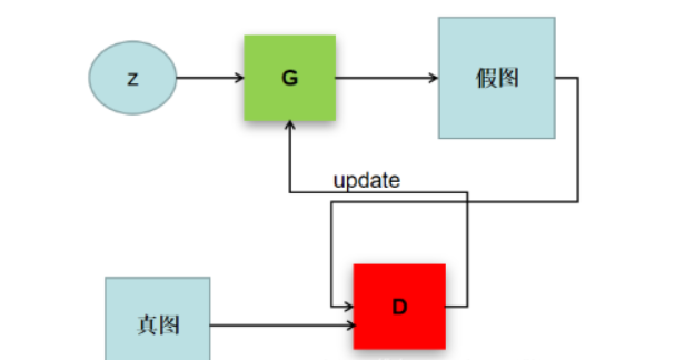
The framework is Generative Adversarial Networks (GAN). A simple understanding is that there are two models in the generation of the antagonistic Network - generators and discriminators. During the training process, two models are trained to play against each other. Finally, a generator that can generate near-real pictures and a judge that can recognize real and virtual pictures are trained.
GAN Variant - DCGAN
DCGAN is a better improvement to GAN. Its main improvement is in the network structure. To date, DCGAN greatly improves the stability of GAN training and the quality of results generated.
The original GAN used the multilayer perception machine as the basic model of generator and judger (of course, in theory, other models can be used as long as the corresponding tasks can be completed), while DCGAN used the convolution neural network as the basic model of generator and judger. Of course, the convolution network used here is different from the usual one. The main changes are as follows:
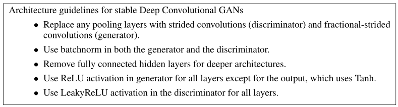
1. Cancel all pooling layers, complete up-sampling with transpose convolution in G and replace with step convolution in D.
2. Batch normalization is used in both generator and adjudicator;
3. Remove the fully connected hidden layer;
4. G uses relu as the activation function, but tanh as the output;
5. The discriminator uses leakyrelu as its activation function.
Training process
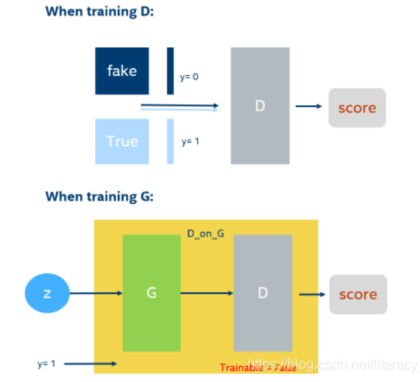
As shown in the figure, when training the discriminator, use the D model directly to train and set different labels for the real and generated data. When training the generator, it is trained directly through the whole generation of the antagonistic network, but the D model is not trainable at this time, and the label should be set to 1 because we want the final output to be that the discriminator recognizes the generated picture as a real picture.
The two models do not train G separately until D is fully trained. They train D simultaneously after a batch, G starts training, G completes a batch, D starts training again, and so on.
Here is only a simple overview of the training process, detailed training process can be referred to Detailed Generate Antagonist Network (GAN).
code implementation
GAN
First import the appropriate Libraries
import tensorflow as tf
import keras
from tensorflow.keras.datasets import mnist
from tensorflow.keras.models import Sequential,Model
from tensorflow.keras.layers import Input,Dense,Dropout,Activation,Flatten
from tensorflow.keras.optimizers import Adam,RMSprop
import numpy as np
import matplotlib.pyplot as plt
import random
Then, import the data and preprocess it, using the MNIST dataset directly here
(x_train, y_train), (x_test, y_test) = mnist.load_data()
x_train = x_train.reshape(60000,784)
x_test = x_test.reshape(10000,784)
x_train = x_train.astype('float32')/255
x_test = x_test.astype('float32')/255
Set the noise level
z_dim = 100
Set up the optimizer, the parameters set in the DCGAN paper referenced here
adam = Adam(lr=0.0002,beta_1=0.5)
Build Generator Model
g = Sequential()
g.add(Dense(256,input_dim=z_dim,activation='relu'))
g.add(Dense(512,activation='relu'))
g.add(Dense(1024,activation='relu'))
g.add(Dense(2048,activation='relu'))
g.add(Dense(784,activation='sigmoid'))
g.compile(loss='binary_crossentropy',optimizer=adam,metrics=['accuracy'])
Build the discriminator model, first set the D model as untrainable, because we need to train the G first
d = Sequential()
d.add(Dense(1024,input_dim=784,activation='relu'))
d.add(Dropout(0.3))
d.add(Dense(512,activation='relu'))
d.add(Dropout(0.3))
d.add(Dense(256,activation='relu'))
d.add(Dropout(0.3))
d.add(Dense(64,activation='relu'))
d.add(Dropout(0.3))
d.add(Dense(1,activation='sigmoid'))
d.compile(loss='binary_crossentropy',optimizer=adam,metrics=['accuracy'])
d.trainable = False
Connect the two models to form an antagonistic network
inputs = Input(shape=(z_dim,))
hidden = g(inputs)
output = d(hidden)
gan = Model(inputs,output)
gan.compile(loss='binary_crossentropy',optimizer=adam,metrics=['accuracy'])
Write two functions for the final output of the loss value and the image generated by the generator
def plot_loss(losses):
    d_loss = [v[0] for v in losses["D"]]
    g_loss = [v[0] for v in losses["G"]]

    plt.figure(figsize=(10,8))
    plt.plot(d_loss,label="Discriminator_loss")
    plt.plot(g_loss,label="Generator_loss")
    plt.legend()
    plt.show()

def plot_generatored(n_ex=10,dim=(1,10),figsize=(12,2)):
    #####
    #np.random.seed(time.time())
    noise = np.random.normal(0,1,size=(n_ex,z_dim))
    generatored_images = g.predict(noise)
    generatored_images = generatored_images.reshape(n_ex,28,28)

    plt.figure(figsize = figsize)
    for i in range(generatored_images.shape[0]):
        plt.subplot(dim[0],dim[1],i+1)
        plt.imshow(generatored_images[i],interpolation='nearest',cmap='gray_r')
        plt.axis('off')
    plt.tight_layout()
    plt.show()
Set up two dictionaries to hold loss values
losses = {"D":[],"G":[]}
Here is the train function
def train(epochs=1,plt_frq=1,BATCH_SIZE=128):
    batchCount = int(x_train.shape[0]/BATCH_SIZE)
    print("Epochs:",epochs)
    print("Batch size:",BATCH_SIZE)
    print("Batches per epoch:",batchCount)

    for e in range(1,epochs+1):
        if e == 1 or e%plt_frq == 0:
            print('-'*15,'Epoch %d' %e,'-'*15)
        for _ in range(batchCount):
            image_batch = x_train[np.random.randint(0,x_train.shape[0],size=BATCH_SIZE)]
            ########
            #np.random.seed(time.time())
            noise = np.random.normal(0,1,size=(BATCH_SIZE,z_dim))
            generatored_images = g.predict(noise)
            #train d
            #set data set which is composed of 2 parts
            x = np.concatenate((image_batch, generatored_images))
            #y are labels
            y = np.zeros(2*BATCH_SIZE)
            y[:BATCH_SIZE] = 0.9

            d.trainable = True
            d_loss = d.train_on_batch(x,y)

            #train g
            #set up data set
            noise = np.random.normal(0,1,size=(BATCH_SIZE,z_dim))
            y2 = np.ones(BATCH_SIZE)
            d.trainable = False
            g_loss = gan.train_on_batch(noise,y2)
        losses["D"].append(d_loss)
        losses["G"].append(g_loss)
        if e==1 or e%plt_frq==0:
            plot_generatored()
    plot_loss(losses)
Then you can start training
train(200,20,128)
Since my previous training data was lost, the GAN results will not be shown here.
DCGAN
I can't copy the results of the paper completely here, just replace the neural network used in the code above with a few points mentioned in the paper and then transform the convolution neural network I used before.
The first step is still to import the related libraries, but this is not needed for some of the above layers
import tensorflow as tf
import keras
from tensorflow.keras.datasets import mnist
from tensorflow.keras.models import Sequential,Model
from tensorflow.keras.layers import Input,Dense,Dropout,Activation,Flatten,Conv2D,Conv2DTranspose,BatchNormalization,LeakyReLU
from tensorflow.keras.optimizers import Adam,RMSprop
import numpy as np
import matplotlib.pyplot as plt
Then import the data and preprocess it as well
(x_train, y_train), (x_test, y_test) = mnist.load_data()
x_train = x_train.reshape(60000,784)
x_test = x_test.reshape(10000,784)
x_train = x_train.astype('float32')/255
x_test = x_test.astype('float32')/255
Setting the noise dimension here uses a different noise dimension than above. When I studied self-encoder before, I found that the dimension of 4_4_8 in the dataset restores handwritten digital pictures very well, so I set it here as well.
z_dim = (4,4,8)
Set up optimizer, same as above
adam = Adam(lr=0.0002,beta_1=0.5)
Build Generator Model
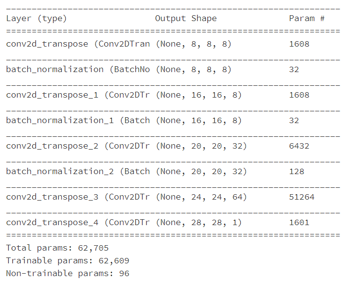
g = Sequential()
g.add(Conv2DTranspose(8,(5,5),activation='relu',input_shape=z_dim))
g.add(BatchNormalization())
g.add(Conv2DTranspose(8,(5,5),activation='relu',strides=2,padding='same'))
g.add(BatchNormalization())
g.add(Conv2DTranspose(32,(5,5),activation='relu'))
g.add(BatchNormalization())
g.add(Conv2DTranspose(64,(5,5),activation='relu'))
g.add(Conv2DTranspose(1,(5,5),activation='tanh'))
g.compile(loss='binary_crossentropy',optimizer=adam,metrics=['accuracy'])
g.summary()
: This is the structure of the G model
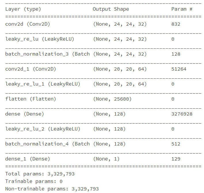
Build Discriminator
d = Sequential()
d.add(Conv2D(32, (5,5),input_shape=(28, 28, 1)))
d.add(LeakyReLU(alpha=0.2))
d.add(BatchNormalization())

d.add(Conv2D(64, (5,5)))
d.add(LeakyReLU(alpha=0.2))

d.add(Flatten())

d.add(Dense(128))
d.add(LeakyReLU(alpha=0.2))

d.add(BatchNormalization())
d.add(Dense(1, activation='softmax'))
d.compile(loss='categorical_crossentropy', optimizer=adam, metrics = ['accuracy'])#Define loss values, optimizers
d.trainable=False
d.summary()
: This is the structure of the discriminator
Similarly, combine the two models to generate a antagonistic network
inputs = Input(shape=(z_dim[0],z_dim[1],z_dim[2],))
hidden = g(inputs)
output = d(hidden)
gan = Model(inputs,output)
gan.compile(loss='binary_crossentropy',optimizer=adam,metrics=['accuracy'])
gan.summary()
Two functions to draw loss values and generator images
def plot_loss(losses):
    d_loss = [v[0] for v in losses["D"]]
    g_loss = [v[0] for v in losses["G"]]

    plt.figure(figsize=(10,8))
    plt.plot(d_loss,label="Discriminator_loss")
    plt.plot(g_loss,label="Generator_loss")
    plt.legend()
    plt.show()

def plot_generatored(n_ex=10,dim=(1,10),figsize=(12,2)):

    noise = np.random.normal(0,1,size=(n_ex,z_dim[0],z_dim[1],z_dim[2]))
    generatored_images = g.predict(noise)
    generatored_images = generatored_images.reshape(n_ex,28,28)

    plt.figure(figsize = figsize)
    for i in range(generatored_images.shape[0]):
        plt.subplot(dim[0],dim[1],i+1)
        plt.imshow(generatored_images[i],interpolation='nearest',cmap='gray_r')
        plt.axis('off')
    plt.tight_layout()
    plt.show()
Set up a dictionary, as above
losses = {"D":[],"G":[]}
train function, same as above
def train(epochs=1,plt_frq=1,BATCH_SIZE=128):
    batchCount = int(x_train.shape[0]/BATCH_SIZE)
    print("Epochs:",epochs)
    print("Batch size:",BATCH_SIZE)
    print("Batches per epoch:",batchCount)

    for e in range(1,epochs+1):
        if e == 1 or e%plt_frq == 0:
            print('-'*15,'Epoch %d' %e,'-'*15)
        for _ in range(batchCount):
            image_batch = x_train[np.random.randint(0,x_train.shape[0],size=BATCH_SIZE)]
            noise = np.random.normal(0,1,size=(BATCH_SIZE,z_dim[0],z_dim[1],z_dim[2]))
            generatored_images = g.predict(noise)
            #train d
            #set data set which is composed of 2 parts
            x = np.concatenate((np.reshape(image_batch,(-1,28,28,1)), generatored_images))
            #y are labels
            y = np.zeros(2*BATCH_SIZE)
            y[:BATCH_SIZE] = 0.9

            d.trainable = True
            d_loss = d.train_on_batch(x,y)

            #train g
            #set up data set
            noise = np.random.normal(0,1,size=(BATCH_SIZE,z_dim[0],z_dim[1],z_dim[2]))
            y2 = np.ones(BATCH_SIZE)
            d.trainable = False
            g_loss = gan.train_on_batch(noise,y2)
        losses["D"].append(d_loss)
        losses["G"].append(g_loss)
        if e==1 or e%plt_frq==0:
            plot_generatored()
    plot_loss(losses)
Then you can start training
train(100,10,128)
Result Display
This is the first image generated:
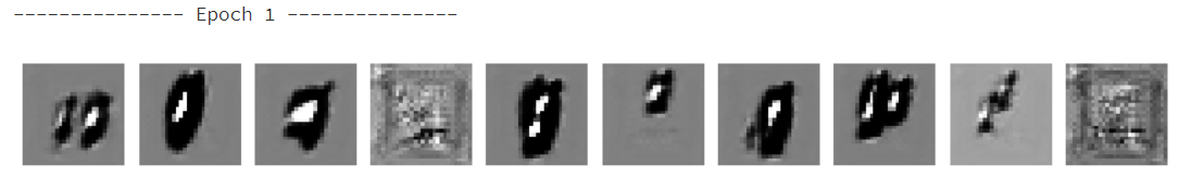
It's so messy that I can't see anything. Maybe my network model is not set up well.
After 10 rounds
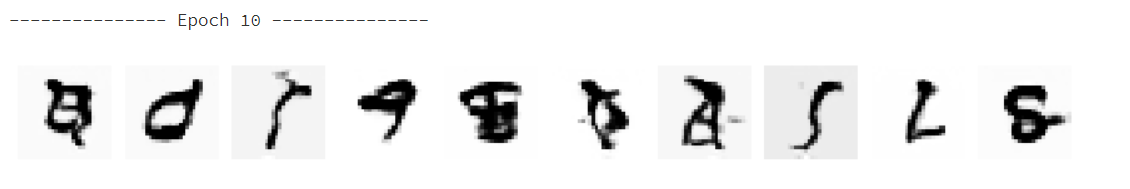
You can see something now, but it's still messy
100 wheels
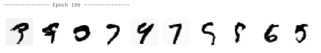
Now you can basically see something, 9, 7, 6, 5 have a strong recognition.
summary
When I first trained DCGAN, I used the usual convolution neural networks directly, including convolution pooling, etc. Generators also used up-sampling instead of transposing convolution. At that time, the computer not only crashed after a very long training period, but also had very poor results.
All code has been published in the whale community Click Direct Can be run directly on it.
When I blog, I refer to a lot of big guys'blogs, and the original articles of GAN and DCGAN are pasted below:
The pictures in the blog are also from here.
Detailed Generate Antagonist Network (GAN)
GAN Generation Conflict Network
Paper:
GAN
DCGAN