matters needing attention
This is the reconstructed deep labv3 + semantic segmentation network, mainly the construction on the file framework and the implementation of code. Compared with the previous semantic segmentation network, it is more complete and clearer. It is recommended to learn this version of DeeplabV3 +.
Study Preface
Deep labv3 + also needs to be refactored!

What is the deep labv3 + model
DeeplabV3 + is considered a new peak of semantic segmentation because the effect of this model is very good.
DeepLabv3 + mainly focuses on the architecture of the model, introduces the resolution that can arbitrarily control the feature extracted by the encoder, and balances the accuracy and time-consuming through hole convolution.
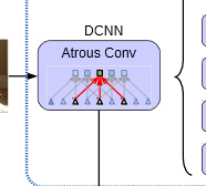
DeeplabV3 + introduces a large number of hole convolutions in the Encoder, and increases the receptive field without losing information, so that each convolution output contains a large range of information. The following is a schematic diagram of hole convolution. The so-called hole is that the feature points will cross pixels when extracted.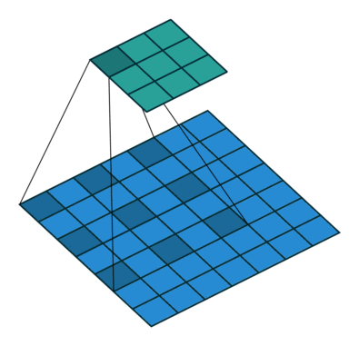
Code download
Github source code download address is:
https://github.com/bubbliiiing/deeplabv3-plus-keras
Copy the path to the address bar to jump.
Deep labv3 + implementation ideas
1, Prediction part
1. Introduction to backbone network
DeeplabV3 + uses Xception series as the backbone feature extraction network in the paper. This blog will provide you with two backbone networks, Xception and mobilenetv2.
However, due to the limitation of computing power (I don't have any cards), in order to facilitate the blog, this paper takes mobilenetv2 as an example to analyze it.
MobileNet model is a lightweight deep neural network proposed by Google for embedded devices such as mobile phones.
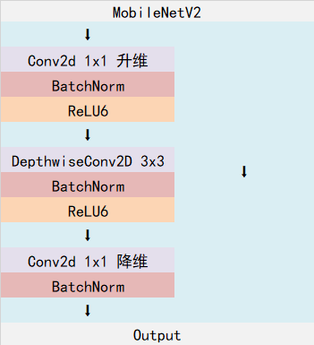
Mobilenetv2 is an upgraded version of MobileNet. It has a very important feature that it uses Inverted resblock. The whole mobilenetv2 is composed of Inverted resblock.
The Inverted resblock can be divided into two parts:
On the left is the main part. Firstly, 1x1 convolution is used for dimension upgrading, then 3x3 depth separable convolution is used for feature extraction, and then 1x1 convolution is used for dimension reduction.
On the right is the residual edge, and the input and output are directly connected.
It should be noted that in DeeplabV3, there are generally not 5 down samples. There are 3 down samples and 4 down samples available. The 4 down samples used in this paper. The down sampling mentioned here means that five times of length and width compression will not be carried out, and three or four times of length and width compression is usually selected.
After completing the feature extraction of MobilenetV2, we can obtain two effective feature layers. One effective feature layer is the result of two times of height and width compression of the input picture, and the other effective feature layer is the result of four times of height and width compression of the input picture.
from keras import layers
from keras.activations import relu
from keras.layers import (Activation, Add, BatchNormalization, Concatenate,
                          Conv2D, DepthwiseConv2D, Dropout,
                          GlobalAveragePooling2D, Input, Lambda, ZeroPadding2D)
from keras.models import Model


def _make_divisible(v, divisor, min_value=None):
    if min_value is None:
        min_value = divisor
    new_v = max(min_value, int(v + divisor / 2) // divisor * divisor)
    if new_v < 0.9 * v:
        new_v += divisor
    return new_v

def relu6(x):
    return relu(x, max_value=6)

def _inverted_res_block(inputs, expansion, stride, alpha, filters, block_id, skip_connection, rate=1):
    in_channels = inputs.shape[-1].value  # inputs._keras_shape[-1]
    pointwise_conv_filters = int(filters * alpha)
    pointwise_filters = _make_divisible(pointwise_conv_filters, 8)
    x = inputs
    prefix = 'expanded_conv_{}_'.format(block_id)
    if block_id:
        # Expand

        x = Conv2D(expansion * in_channels, kernel_size=1, padding='same',
                   use_bias=False, activation=None,
                   name=prefix + 'expand')(x)
        x = BatchNormalization(epsilon=1e-3, momentum=0.999,
                               name=prefix + 'expand_BN')(x)
        x = Activation(relu6, name=prefix + 'expand_relu')(x)
    else:
        prefix = 'expanded_conv_'
    # Depthwise
    x = DepthwiseConv2D(kernel_size=3, strides=stride, activation=None,
                        use_bias=False, padding='same', dilation_rate=(rate, rate),
                        name=prefix + 'depthwise')(x)
    x = BatchNormalization(epsilon=1e-3, momentum=0.999,
                           name=prefix + 'depthwise_BN')(x)

    x = Activation(relu6, name=prefix + 'depthwise_relu')(x)

    # Project
    x = Conv2D(pointwise_filters,
               kernel_size=1, padding='same', use_bias=False, activation=None,
               name=prefix + 'project')(x)
    x = BatchNormalization(epsilon=1e-3, momentum=0.999,
                           name=prefix + 'project_BN')(x)

    if skip_connection:
        return Add(name=prefix + 'add')([inputs, x])

    # if in_channels == pointwise_filters and stride == 1:
    #    return Add(name='res_connect_' + str(block_id))([inputs, x])

    return x

def mobilenetV2(inputs, alpha=1, downsample_factor=8):
    if downsample_factor == 8:
        block4_dilation = 2
        block5_dilation = 4
        block4_stride = 1
        atrous_rates = (12, 24, 36)
    elif downsample_factor == 16:
        block4_dilation = 1
        block5_dilation = 2
        block4_stride = 2
        atrous_rates = (6, 12, 18)
    else:
        raise ValueError('Unsupported factor - `{}`, Use 8 or 16.'.format(downsample_factor))

    first_block_filters = _make_divisible(32 * alpha, 8)
    # 512,512,3 -> 256,256,32
    x = Conv2D(first_block_filters,
                kernel_size=3,
                strides=(2, 2), padding='same',
                use_bias=False, name='Conv')(inputs)
    x = BatchNormalization(
        epsilon=1e-3, momentum=0.999, name='Conv_BN')(x)
    x = Activation(relu6, name='Conv_Relu6')(x)


    x = _inverted_res_block(x, filters=16, alpha=alpha, stride=1,
                            expansion=1, block_id=0, skip_connection=False)

    #---------------------------------------------------------------#
    # 256,256,16 -> 128,128,24
    x = _inverted_res_block(x, filters=24, alpha=alpha, stride=2,
                            expansion=6, block_id=1, skip_connection=False)
    x = _inverted_res_block(x, filters=24, alpha=alpha, stride=1,
                            expansion=6, block_id=2, skip_connection=True)
    skip1 = x
    #---------------------------------------------------------------#
    # 128,128,24 -> 64,64.32
    x = _inverted_res_block(x, filters=32, alpha=alpha, stride=2,
                            expansion=6, block_id=3, skip_connection=False)
    x = _inverted_res_block(x, filters=32, alpha=alpha, stride=1,
                            expansion=6, block_id=4, skip_connection=True)
    x = _inverted_res_block(x, filters=32, alpha=alpha, stride=1,
                            expansion=6, block_id=5, skip_connection=True)
    #---------------------------------------------------------------#
    # 64,64,32 -> 32,32.64
    x = _inverted_res_block(x, filters=64, alpha=alpha, stride=block4_stride,
                            expansion=6, block_id=6, skip_connection=False)
    x = _inverted_res_block(x, filters=64, alpha=alpha, stride=1, rate=block4_dilation,
                            expansion=6, block_id=7, skip_connection=True)
    x = _inverted_res_block(x, filters=64, alpha=alpha, stride=1, rate=block4_dilation,
                            expansion=6, block_id=8, skip_connection=True)
    x = _inverted_res_block(x, filters=64, alpha=alpha, stride=1, rate=block4_dilation,
                            expansion=6, block_id=9, skip_connection=True)

    # 32,32.64 -> 32,32.96
    x = _inverted_res_block(x, filters=96, alpha=alpha, stride=1, rate=block4_dilation,
                            expansion=6, block_id=10, skip_connection=False)
    x = _inverted_res_block(x, filters=96, alpha=alpha, stride=1, rate=block4_dilation,
                            expansion=6, block_id=11, skip_connection=True)
    x = _inverted_res_block(x, filters=96, alpha=alpha, stride=1, rate=block4_dilation,
                            expansion=6, block_id=12, skip_connection=True)

    #---------------------------------------------------------------#
    # 32,32.96 -> 32,32,160 -> 32,32,320
    x = _inverted_res_block(x, filters=160, alpha=alpha, stride=1, rate=block4_dilation,  # 1!
                            expansion=6, block_id=13, skip_connection=False)
    x = _inverted_res_block(x, filters=160, alpha=alpha, stride=1, rate=block5_dilation,
                            expansion=6, block_id=14, skip_connection=True)
    x = _inverted_res_block(x, filters=160, alpha=alpha, stride=1, rate=block5_dilation,
                            expansion=6, block_id=15, skip_connection=True)

    x = _inverted_res_block(x, filters=320, alpha=alpha, stride=1, rate=block5_dilation,
                            expansion=6, block_id=16, skip_connection=False)
    return x,atrous_rates,skip1
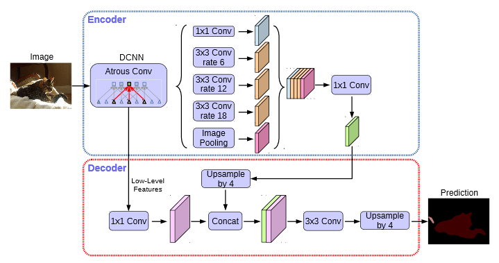
2. Strengthen feature extraction structure
In DeeplabV3 +, the enhanced feature extraction network can be divided into two parts:
In the Encoder, we will use the parallel atrus revolution for the preliminary effective feature layer compressed four times, extract the features with atrus revolution of different rate s, merge them, and then 1x1 convolution compress the features.
In the Decoder, we will use 1x1 convolution to adjust the number of channels for the preliminary effective feature layer compressed twice, and then stack with the sampling results on the effective feature layer after hole convolution. After stacking, we will perform two deep separable convolution blocks.
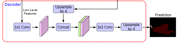
At this time, we get a final effective feature layer, which is the feature concentration of the whole picture.
def Deeplabv3(n_classes, inputs_size, alpha=1., backbone="mobilenet", downsample_factor=16):
    img_input = Input(shape=inputs_size)

    if backbone=="xception":
        x,atrous_rates,skip1 = Xception(img_input,alpha, downsample_factor=downsample_factor)
    elif backbone=="mobilenet":
        x,atrous_rates,skip1 = mobilenetV2(img_input,alpha, downsample_factor=downsample_factor)
    else:
        raise ValueError('Unsupported backbone - `{}`, Use mobilenet, xception.'.format(backbone))

    size_before = tf.keras.backend.int_shape(x)

    # Adjust channel
    b0 = Conv2D(256, (1, 1), padding='same', use_bias=False, name='aspp0')(x)
    b0 = BatchNormalization(name='aspp0_BN', epsilon=1e-5)(b0)
    b0 = Activation('relu', name='aspp0_activation')(b0)

    # rate = 6 (12)
    b1 = SepConv_BN(x, 256, 'aspp1',
                    rate=atrous_rates[0], depth_activation=True, epsilon=1e-5)
    # rate = 12 (24)
    b2 = SepConv_BN(x, 256, 'aspp2',
                    rate=atrous_rates[1], depth_activation=True, epsilon=1e-5)
    # rate = 18 (36)
    b3 = SepConv_BN(x, 256, 'aspp3',
                    rate=atrous_rates[2], depth_activation=True, epsilon=1e-5)

    # After all are averaged, expand is used_ Dims extended dimension, 1x1
    # shape = 320
    b4 = GlobalAveragePooling2D()(x)
    b4 = Lambda(lambda x: K.expand_dims(x, 1))(b4)
    b4 = Lambda(lambda x: K.expand_dims(x, 1))(b4)

    # Compression filter
    b4 = Conv2D(256, (1, 1), padding='same', use_bias=False, name='image_pooling')(b4)
    b4 = BatchNormalization(name='image_pooling_BN', epsilon=1e-5)(b4)
    b4 = Activation('relu')(b4)

    # Direct use of resize_images extension hw
    b4 = Lambda(lambda x: tf.image.resize_images(x, size_before[1:3], align_corners=True))(b4)

    x = Concatenate()([b4, b0, b1, b2, b3])

    # Using conv2d compression
    # 32,32,256
    x = Conv2D(256, (1, 1), padding='same',
               use_bias=False, name='concat_projection')(x)
    x = BatchNormalization(name='concat_projection_BN', epsilon=1e-5)(x)
    x = Activation('relu')(x)
    x = Dropout(0.1)(x)

    # x4 (x2) block
    skip_size = tf.keras.backend.int_shape(skip1)
    x = Lambda(lambda xx: tf.image.resize_images(xx, skip_size[1:3], align_corners=True))(x)

    dec_skip1 = Conv2D(48, (1, 1), padding='same',use_bias=False, name='feature_projection0')(skip1)
    dec_skip1 = BatchNormalization(name='feature_projection0_BN', epsilon=1e-5)(dec_skip1)
    dec_skip1 = Activation(tf.nn.relu)(dec_skip1)

    x = Concatenate()([x, dec_skip1])
    x = SepConv_BN(x, 256, 'decoder_conv0',
                    depth_activation=True, epsilon=1e-5)
    x = SepConv_BN(x, 256, 'decoder_conv1',
                    depth_activation=True, epsilon=1e-5)
3. Using features to obtain prediction results
Using steps 1 and 2, we can obtain the features of the input picture. At this time, we need to use the features to obtain the prediction results.
The process of using features to obtain prediction results can be divided into two steps:
1. Use a 1x1 convolution to adjust the channel to Num_Classes.
2. Use resize for up sampling, so that the width and height of the final output layer are the same as those of the input picture.
from keras.models import *
from keras.layers import *
from nets.mobilenetv2 import get_mobilenet_encoder
from nets.resnet50 import get_resnet50_encoder
import tensorflow as tf

IMAGE_ORDERING = 'channels_last'
MERGE_AXIS = -1

def resize_image(inp, s, data_format):
	return Lambda(lambda x: tf.image.resize_images(x, (K.int_shape(x)[1]*s[0], K.int_shape(x)[2]*s[1])))(inp)

def pool_block(feats, pool_factor, out_channel):
	h = K.int_shape(feats)[1]
	w = K.int_shape(feats)[2]
	# strides = [30,30],[15,15],[10,10],[5,5]
	pool_size = strides = [int(np.round(float(h)/pool_factor)),int(np.round(float(w)/pool_factor))]
	# Average in different degrees
	x = AveragePooling2D(pool_size , data_format=IMAGE_ORDERING , strides=strides, padding='same')(feats)
	# Convolution
	x = Conv2D(out_channel//4, (1 ,1), data_format=IMAGE_ORDERING, padding='same', use_bias=False)(x)
	x = BatchNormalization()(x)
	x = Activation('relu' )(x)
	x = Lambda(lambda x: tf.image.resize_images(x, (K.int_shape(feats)[1], K.int_shape(feats)[2]), align_corners=True))(x)
	return x

def pspnet(n_classes, inputs_size, downsample_factor=8, backbone='mobilenet', aux_branch=True):
	if backbone == "mobilenet":
		img_input, f4, o = get_mobilenet_encoder(inputs_size, downsample_factor=downsample_factor)
		out_channel = 320
	elif backbone == "resnet50":
		img_input, f4, o = get_resnet50_encoder(inputs_size, downsample_factor=downsample_factor)
		out_channel = 2048
	else:
		raise ValueError('Unsupported backbone - `{}`, Use mobilenet, resnet50.'.format(backbone))

	# Pool to varying degrees
	pool_factors = [1,2,3,6]
	pool_outs = [o]

	for p in pool_factors:
		pooled = pool_block(o, p, out_channel)
		pool_outs.append(pooled)

	# connect
	# 60x60x
	o = Concatenate(axis=MERGE_AXIS)(pool_outs)

	# convolution
	# 60x60x512
	o = Conv2D(out_channel//4, (3,3), data_format=IMAGE_ORDERING, padding='same', use_bias=False)(o)
	o = BatchNormalization()(o)
	o = Activation('relu')(o)
	o = Dropout(0.1)(o)

	# 60x60x21
	o = Conv2D(n_classes,(1,1),data_format=IMAGE_ORDERING, padding='same')(o)
	# [473,473,nclasses]
	o = Lambda(lambda x: tf.image.resize_images(x, (inputs_size[1], inputs_size[0]), align_corners=True))(o)
	o = Activation("softmax", name="main")(o)

	if aux_branch:
		f4 = Conv2D(out_channel//8, (3,3), data_format=IMAGE_ORDERING, padding='same', use_bias=False)(f4)
		f4 = BatchNormalization()(f4)
		f4 = Activation('relu')(f4)
		f4 = Dropout(0.1)(f4)

		# 60x60x21
		f4 = Conv2D(n_classes,(1,1),data_format=IMAGE_ORDERING, padding='same')(f4)
		# [473,473,nclasses]
		f4 = Lambda(lambda x: tf.image.resize_images(x, (inputs_size[1], inputs_size[0]), align_corners=True))(f4)
		f4 = Activation("softmax", name="aux")(f4)
		model = Model(img_input,[f4,o])
		return model
	else:
		model = Model(img_input,[o])
		return model
2, Training part
1. Detailed explanation of training documents
The training files we use are in VOC format.
The training file of semantic segmentation model is divided into two parts.
The first part is the original drawing, like this:
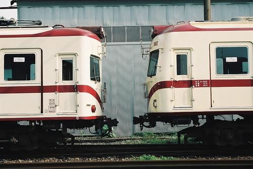
Part II label, like this:

The original image is an ordinary RGB image, and the label is a grayscale image or an 8-bit color image.
The shape of the original image is [height, width, 3], and the shape of the label is [height, width]. For the label, the content of each pixel is a number, such as 0, 1, 2, 3, 4, 5... Representing the category to which the pixel belongs.
The work of semantic segmentation is to classify each pixel of the original picture, so the network can be trained by comparing the probability of each pixel belonging to each category in the prediction result with the label.
2. LOSS analysis
LOSS used in this article consists of two parts:
1,Cross Entropy Loss.
2,Dice Loss.
Cross Entropy Loss is a common Cross Entropy Loss. It is used when the semantic segmentation platform uses Softmax to classify pixels.
Dice loss takes the evaluation index of semantic segmentation as Loss. Dice coefficient is a set similarity measurement function, which is usually used to calculate the similarity between two samples, and the value range is [0,1].
The calculation formula is as follows:
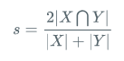
Is the intersection of the predicted result and the real result multiplied by 2, divided by the predicted result and the real result. Its value is between 0-1. The larger the value, the greater the coincidence between the predicted results and the real results. So the larger the Dice coefficient, the better.
If it is used as loss, the smaller the better, so if Dice loss = 1 - Dice, loss can be used as the loss of semantic segmentation.
The implementation code is as follows:
def dice_loss_with_CE(beta=1, smooth = 1e-5):
    def _dice_loss_with_CE(y_true, y_pred):
        y_pred = K.clip(y_pred, K.epsilon(), 1.0 - K.epsilon())

        CE_loss = - y_true[...,:-1] * K.log(y_pred)
        CE_loss = K.mean(K.sum(CE_loss, axis = -1))

        tp = K.sum(y_true[...,:-1] * y_pred, axis=[0,1,2])
        fp = K.sum(y_pred         , axis=[0,1,2]) - tp
        fn = K.sum(y_true[...,:-1], axis=[0,1,2]) - tp

        score = ((1 + beta ** 2) * tp + smooth) / ((1 + beta ** 2) * tp + beta ** 2 * fn + fp + smooth)
        score = tf.reduce_mean(score)
        dice_loss = 1 - score
        # dice_loss = tf.Print(dice_loss, [dice_loss, CE_loss])
        return CE_loss + dice_loss
    return _dice_loss_with_CE
Train your own DeeplabV3 + model
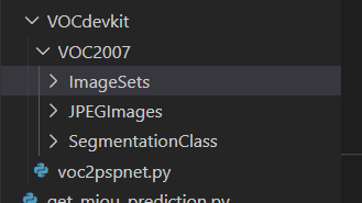
The file architecture of the whole DeeplabV3 + is:
Before training the model, we need to prepare the data set first.
You can download the voc dataset I uploaded, or make the dataset according to the voc dataset format.
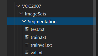
If you download the VOC dataset I uploaded, you don't need to run voc2deeplab. Under the VOCdevkit folder py.
If the dataset is made by yourself, you need to run voc2deeplab. Under the VOCdevkit folder Py to generate train Txt and val.txt.
When the build is complete.
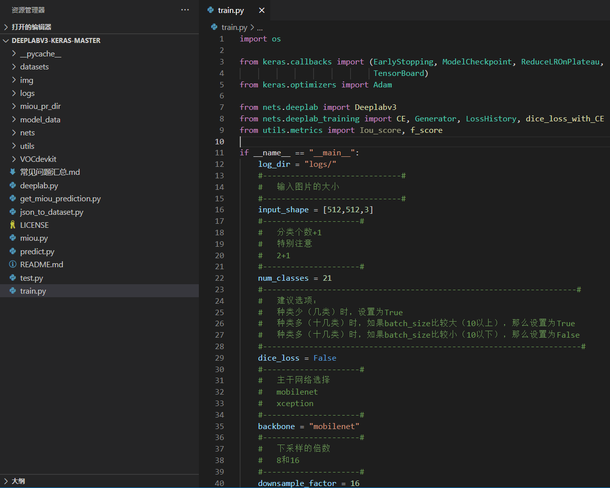
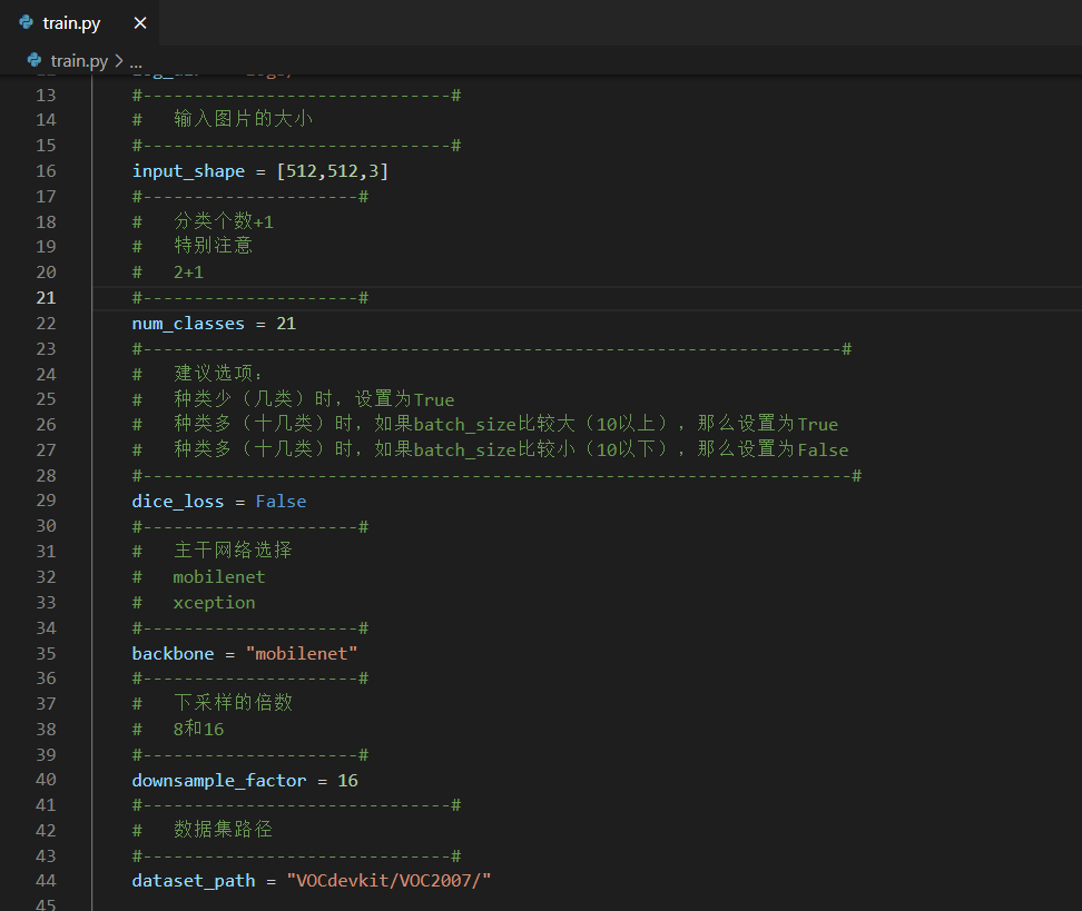
In train Py folder, select the trunk model and down sampling factor you want to use.
The backbone models provided in this paper are mobilenet and xception.
The down sampling factor can be selected from 8 and 16.
It should be noted that the pre training model should correspond to the trunk model.
Then you can start training.