Introduction to sklearn -- implementation of regression decision tree in sklearn_ Example demonstration 1

1. Introduction to regression tree

Almost all parameters in as like as two peas are categorization. The parameters of the regression tree function are as follows:

class sklearn.tree.DecisionTreeRegressor (criterion='mse', splitter='best', max_depth=None,min_samples_split=2, min_samples_leaf=1, min_weight_fraction_leaf=0.0, max_features=None,random_state=None, max_leaf_nodes=None, min_impurity_decrease=0.0, min_impurity_split=None, presort=False)

2. Important parameters, attributes and interfaces

criterion: the regression tree is an indicator to measure the quality of branches. There are three types of criteria supported:

• Enter "mse" to use mean square error (mse), and the difference between the mean square error of the parent node and the leaf node will be used as

  This method minimizes L2 loss by using the mean of leaf nodes.

• Enter "friedman_mse" to use Feldman mean square error, which uses Friedman's improved mean square error for problems in potential branching.

• Enter "MAE" to use the absolute mean error MAE (mean absolute error), which uses the median of leaf nodes to minimize L1 loss.

The most important attribute is feature_importances_， Is used to view the importance of attributes.

The most important interfaces are: apply, fit, predict and score.

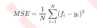
Where N is the number of samples, i is each data sample, fifi is the value regressed by the model, and yi is the actual value label of sample point i. MSE is actually the difference between sample real data and regression results. In regression, what we pursue is that the smaller the MSE, the better. Because the smaller the MSE, the smaller the difference between the predicted value and the actual value, and the prediction is more accurate.

However, the regression tree interface score returns r square, not MSE. R squared is defined as follows:

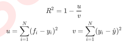
Where u is the sum of squares of residuals (MSE * N), v is the sum of squares, N is the number of samples, i is each data sample, fifi is the value regressed by the model, and yi is the actual value label of sample point i. The y cap is the average number of real value labels. R square can be positive or negative (if the sum of residual squares of the model is much greater than the total sum of squares of the model, the model is very bad, R square will be negative), and the mean square error will always be positive.

It is worth mentioning that although the mean square error is always positive, when the mean square error is used as the evaluation standard in sklearn, it is to calculate the negative mean square error (neg_mean_squared_error). This is because when sklearn calculates the model evaluation index, it will consider the nature of the index itself. The mean square error itself is an error, so it is divided into a loss of the model by sklearn. Therefore, in sklearn, it is expressed as a negative number. The true mean square error MSE is actually NEG_ mean_ squared_ Error remove the number with the minus sign.

3. Regression tree in sklearn

from sklearn.datasets import load_boston  #Import Boston house price dataset
from sklearn.model_selection import cross_val_score  #Import cross validation
from sklearn.tree import DecisionTreeRegressor  #Import regression tree
boston = load_boston()  #Assign the boston dataset to the variable boston
regressor = DecisionTreeRegressor(random_state=0)  #Generate regression tree
cross_val_score(regressor, boston.data, boston.target, cv=10, 
                scoring = "neg_mean_squared_error") #Cross validation_ val_ Usage of score

This is a simple call. When dealing with boston, we can use numpy's knowledge to simply view the data.

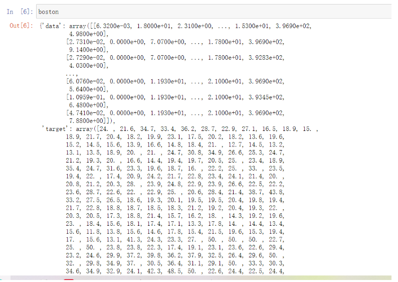
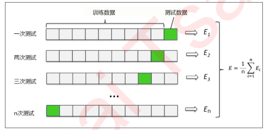
You can see that the data returned by entering boston is in the form of a dictionary. We can also enter boston Data to view features and boston Target and target value. Cross validation is a method used to observe the stability of the model. We divide the data into N parts, use one part as the test set and the other n-1 parts as the training set, and calculate the accuracy of the model for many times to evaluate the average accuracy of the model. The division of training set and test set will interfere with the results of the model, so the average value obtained from the results of cross validation n times is a better measure of the effect of the model.

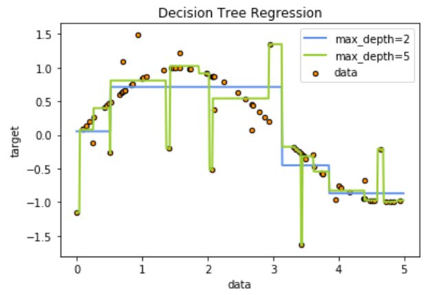
4. Example: image rendering of one-dimensional regression

4.1 import required libraries

import numpy as np #Used to process data quickly
from sklearn.tree import DecisionTreeRegressor
import matplotlib.pyplot as plt #Used to draw pictures

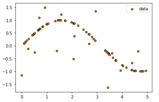
4.2 create a sinusoidal curve with noise

In this step, our basic idea is to create a group of random values (x) of abscissa axis distributed on 0 ~ 5, then put this group of values into sin function to generate the value (y) of ordinate, and then add noise to y. Throughout the process, we will use the numpy library to generate this sine for us.

rng = np.random.RandomState(1)
X = np.sort(5 * rng.rand(80,1), axis=0)#axis=0 means calculated by row, and axis=1 means calculated by column.
#rng.rand(80,1) generates 80 points with a value of 0-1, and then multiplies it by 5 to enlarge the value of the points to 0-5.
#Then use the sort function to sort the rows from large to small.
y = np.sin(X).ravel()#np.sin(x) is two-dimensional data. Use travel () to change the data into one-dimensional data for normal input into the regression tree.
y[::5] += 3 * (0.5 - rng.rand(16)) #For 80 data points, take one value for each five points and add noise.
#Y [start point: end point: step size] y[::5] indicates from start to end, with a step size of 5.
#80 points, 16 points in total, 0.5 - RNG The range of rand (16) is - 0.5 ~ 0.5.

4.3 instantiation and training model

regr_1 = DecisionTreeRegressor(max_depth=2) #The depth of the tree is 2
regr_2 = DecisionTreeRegressor(max_depth=5) #The depth of the tree is 5
regr_1.fit(X, y) #Conduct training
regr_2.fit(X, y)

4.4 test set import model and forecast results

X_test = np.arange(0.0, 5.0, 0.01)[:, np.newaxis]
#np. Array (start point, end point, step size) function to generate an ordered array
y_1 = regr_1.predict(X_test)
y_2 = regr_2.predict(X_test)

4.5 drawing images

plt.figure()
plt.scatter(X, y, s=20, edgecolor="black",c="darkorange", label="data")
plt.plot(X_test, y_1, color="cornflowerblue",label="max_depth=2", linewidth=2)
plt.plot(X_test, y_2, color="yellowgreen", label="max_depth=5", linewidth=2)
plt.xlabel("data")
plt.ylabel("target")
plt.title("Decision Tree Regression")
plt.legend()
plt.show()