1. General
1.1 introduction of convolutional neural network
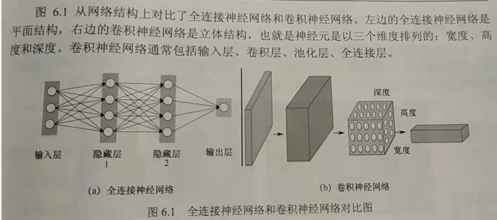
In the previous blog, we made an implementation of fully connected neural network. Among them, the input layer has 784 (28 * 28 picture) elements, the four hidden layers have 400, 300, 200 and 100 neurons respectively, and the output layer includes 10 categories of handwritten digits. The weight required to express such a small neural network is about 520200 (784 * 400 + 300 * 200 + 200 * 100 + 100 * 10). If each weight is represented by a 4-byte floating-point number, These weights will occupy 2080800 bytes, about 1.98MB, which exceeds the memory size of the computer at that time.
Therefore, people began to consider whether the connection mode of fully connected neural network can be changed, which is the emergence of feedforward neural network. Convolutional neural network is a feedforward neural network with convolution operation and depth structure. The reason for the success of convolutional neural network lies in the way of local connection and weight sharing. On the one hand, it reduces the number of weights and makes the network easy to optimize. On the other hand, it reduces the complexity of the model, that is, it reduces the risk of over fitting. Convolutional neural network has excellent performance in large-scale image processing.
1.2 basic criteria of convolutional neural network
1.2.1 locality
It refers to determining the category of a picture by detecting local features in the picture
1.2.2 similarity
It refers to detecting whether different pictures have the same features. Although these features may appear in different places, they can still be judged by local features.
1.2.3 invariance
It refers to the down sampling of a picture (for a sample value sequence, take samples every few samples, so that the new sequence is the down sampling of the original sequence), and the nature of the picture remains basically unchanged
Based on the above three criteria, a typical convolutional neural network consists of at least four parts: input layer, convolution layer, pooling layer and full connection layer. The convolution layer is responsible for extracting the local features of the picture; The pool layer is used to greatly reduce the order of magnitude of parameters (dimension reduction); The full connection layer is similar to the traditional neural network, which is not used to output the prediction results.
2. Network hierarchy analysis
2.1 convolution
Given an image, CNN can not accurately know which parts of the original image these features want to match, so it will try at every possible position in the original image, which is equivalent to treating these features as a filter (also known as convolution kernel). This matching process is called convolution. Different from the fully connected neural network, each neuron in the convolutional neural network is only connected with a local region of the input data, because the filter extracts local features. The size of the space connected to the neurons (i.e. the size of the sensory field, i.e. the width and height of the filter) needs to be set manually.
2.1.1 height and width of filter
The work of each filter is to find a feature in the input data. The width and height of each filter are relatively small, but the depth is consistent with the depth of the input data.
2.1.2 step size
The step size represents the distance each filter moves
2.1.3 boundary filling
Convolution operation will make the size of the convoluted picture smaller and smaller, and because the elements in the upper left corner of the picture are only used by one output, the pixels at the edge of the picture will be less used in the output, which means that a lot of edge information will be lost. In order to solve these two problems, boundary filling (padding operation) is introduced, that is, 0 is used to fill the boundary along the edge of the picture before the image convolution operation. When the step size is equal to 1, filling with 0 can make the input and output data have the same space size.
Set the input picture size to
 , step size s, boundary fill size p, filter size
 , the size of the output picture is
 The calculation formula is as follows:
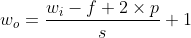
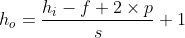

When the size of the input picture is 5 * 5 * 3, the filter size is 3 * 3, the step size is 1, and the size of the boundary filling is 0, the size of the output picture can be calculated as 3 * 3 * 3.
Convolution is the matrix inner product of filter and input picture. The convolution process of a single channel is shown in the figure below:
Using parameter sharing in convolution layer can effectively reduce the number of parameters. The reason why parameters can be shared is that the features are the same, that is, a feature is the same in different locations. Parameter sharing includes shared filter and shared weight vector. Convolution usually uses torch in pytorque nn. To implement the conv2d() function, you first need to enter a torch autograd. The size of variable is (batch, channel,H,W), where batch represents the number of input pictures, channel represents the number of channels of input pictures, and H and W represent the height and width of input pictures. For example, if 32 color pictures are input, the height and width of pictures are 50100 respectively, then the size of input variable is (32, 3, 50100)
2.1.4 implementation of convolution code
from PIL import Image
import numpy as np
import matplotlib.pyplot as plt
import torch
from torch import nn
from torch.autograd import Variable

im = Image.open(r'E:\kaggleData\dog\images\Images\n02085620-Chihuahua\n02085620_199.jpg').convert('L') # Convert to grayscale image
im = np.array(im, dtype='float32') # Convert it into a matrix
plt.imshow(im.astype('uint'), cmap='gray')
plt.show()

# Transform the picture matrix into tensor in PyTorch and adapt to the requirements of convolution input
"""
    Convolution in PyTorch Usually used in torch.nn.Conv2d()Function implementation. First, you need to enter a torch.autograd.Variable Variable of type
 Its size is( batch,channels, H, W)among batch Indicates the number of input pictures, channels Indicates the number of channels for the input picture
 Generally, the number of channels for color pictures is 3, and the number of channels for gray pictures is 1. In the process of convolution, the number of channels will be large, and there will be dozens to hundreds of channels.
"""
im = torch.from_numpy(im.reshape((1, 1, im.shape[0], im.shape[1])))
# Use Conv2d() function
conv1 = nn.Conv2d(1, 1, 3, bias=False)
# Define contour check operator
sobel_kernel = np.array([[-1, -1, -1], [-1, 8, -1], [-1, -1, -1]], dtype='float32')
# Adaptive convolution input / output
sobel_kernel = sobel_kernel.reshape((1, 1, 3, 3))
# Assign a value to the convolution kernel of convolution
conv1.weight.data = torch.from_numpy(sobel_kernel)
# Act on pictures
edge1 = conv1(Variable(im))
# Convert output to picture format
edge1 = edge1.data.squeeze().numpy()
plt.imshow(edge1, cmap='gray')
plt.show()
2.2 pool layer
2.2.1 overview of pool layer
Like the convolution layer, the pooling layer also processes local areas. The pooling layer uses a spatial window (filter), and usually takes the maximum value / weighted average value in these spatial windows as the output result. Then continuously slide the window to process each convolution operation result of the input picture separately to reduce its size space. The functions of pool layer are as follows:
1. Feature dimensionality reduction to avoid over fitting
The image after convolution operation will contain many features, so it is necessary to reduce the dimension of the features through the pooling layer, which is also called down sampling.
2. Space invariance
The pool layer can keep its characteristics unchanged when the picture space changes (rotation, compression, translation). For example, in a picture of a dog, the dog is very clear when there are many pixels. After compressing the picture, the dog becomes smaller, but it can still be seen that there is a dog in the picture, and its main characteristics have not changed.
3. Reduce parameters and training difficulty
Pool processing is generally divided into maximum pool and average pool. Maximum pool is to take the maximum value in the pool space window, and average pool is to take the weighted average value in the pool space window.
NN is commonly used in PyTorch Maxpool2d() function realizes the maximum pool processing. The requirements of this function for input pictures are the same as torch nn. Same as conv2d() function
2.2.2 realization of pool layer
from PIL import Image
import numpy as np
import matplotlib.pyplot as plt
import torch
from torch import nn
from torch.autograd import Variable
# Read a color picture and convert it into a grayscale picture
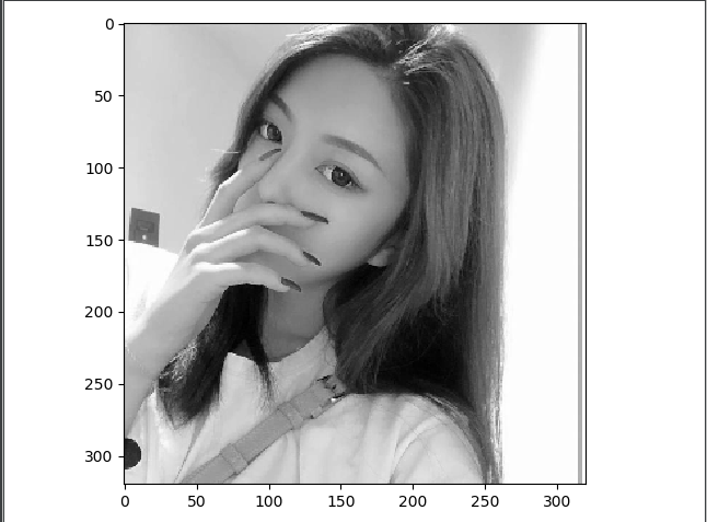
im = Image.open(r'E:\kaggleData\computer_version_Data\test.jpg').convert('L')
# Convert to matrix
im = np.array(im, dtype='float32')
"""
Python There are three functions and attributes related to data types in: type/dtype/astype.
type() Returns the data type of the parameter
dtype Returns the data type of the element in the array
astype() Convert data types
"""
plt.imshow(im.astype('uint8'), cmap='gray')
plt.show()
# The image matrix is transformed into tensor and adapted to the requirements of convolution input
im = torch.from_numpy(im.reshape((1, 1, im.shape[0], im.shape[1])))
pool1 = nn.MaxPool2d(2, 2)
print('before max pool, image shape:{} x {}'.format(im.shape[2], im.shape[3]))
small_im1 = pool1(Variable(im))
# Convert output to picture format
small_im1 = small_im1.data.squeeze().numpy()
print('after max poolm, image shape:{} x {}'.format(small_im1.shape[0], small_im1.shape[1]))
plt.imshow(small_im1, cmap='gray')
plt.show()
The left figure is before the maximum pool, and the right figure is the result after the maximum pool.
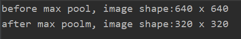
You can see that the pooled image is still very clear.
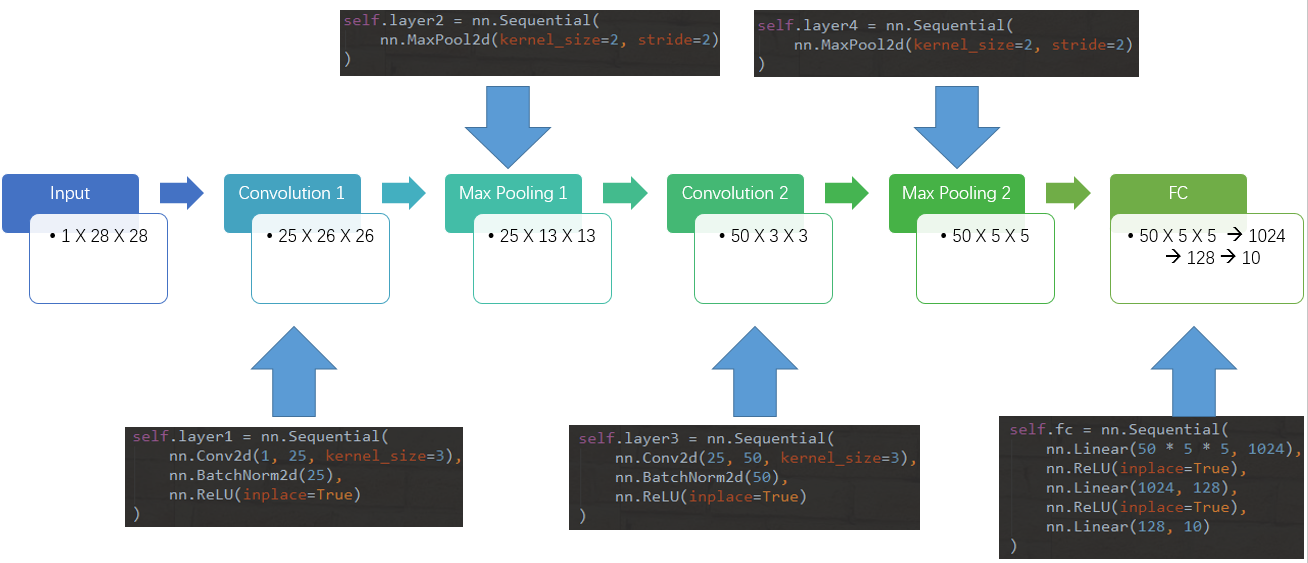
3. Recognition of handwritten digits by convolution neural network based on PyTorch
A total of five layers are defined, including two convolution layers, two pooling layers, and the last layer is FC layer for classified output. Its network structure is as follows:
# package
import torch
import torch.nn as nn
import torch.nn.functional as F
import torch.utils.data as Data

# Torch vision package contains several important public data sets, network models and image transformations commonly used in computer vision
import torchvision
import torchvision.transforms as transforms

import matplotlib.pyplot as plt
import numpy as np

# Equipment configuration
#torch.cuda.set_device(1) # This sentence is used to set which GPU pytorch runs on
#device = torch.device('cuda' if torch.cuda.is_available() else 'cpu')

# Super parameter setting
num_epochs = 5
num_classes = 10
batch_size = 64  # The size of a batch
image_size = 28  #Total size of image 28 * 28
learning_rate = 0.001

# transform=transforms.ToTensor(): convert the image into Tensor, and preprocess the image when loading data
train_dataset = torchvision.datasets.MNIST(root='./data',train=True,transform=transforms.ToTensor(),download=True)
test_dataset = torchvision.datasets.MNIST(root='./data',train=False,transform=transforms.ToTensor(),download=True)

# The loader of the training data set automatically divides the data into batch es and randomly disrupts the order
train_loader = torch.utils.data.DataLoader(dataset=train_dataset,batch_size=batch_size,shuffle=True)
print('len(train_loader):',len(train_loader))
print('len(train_loader.dataset):',len(train_loader.dataset))

"""
Next, take the first 5000 samples in the test data as the verification set and the last 5000 samples as the test set
"""
indices = range(len(test_dataset))
indices_val = indices[:5000]
indices_test = indices[5000:]

# The validation set and test set are sampled by subscript
sampler_val = torch.utils.data.sampler.SubsetRandomSampler(indices_val)
sampler_test = torch.utils.data.sampler.SubsetRandomSampler(indices_test)

# Define the loader according to the sampler, and then load the data
validation_loader = torch.utils.data.DataLoader(dataset =test_dataset,batch_size = batch_size,sampler = sampler_val)

test_loader = torch.utils.data.DataLoader(dataset=test_dataset,batch_size=batch_size,sampler = sampler_test)

#Read a picture from the dataset and draw it
idx = 0
#dataset supports subscript index. Each extracted element is in the format of features and target, that is, attributes and labels. [0] indicates index features
muteimg = train_dataset[idx][0].numpy()
#Because the general image contains rgb three channels, while the images of MINST dataset are grayscale and have only one channel. Therefore, we ignore the channel and treat the image as a gray matrix.

#When drawing with imshow, the gray matrix will be automatically displayed as color. Different gray levels correspond to different colors: from yellow to purple

plt.imshow(muteimg[0,...])
print('The label is:',train_dataset[idx][1])

# Define the thickness of the two convolution layers (number of feature map s)
depth = [4, 8]


class ConvNet(nn.Module):
    def __init__(self):
        super().__init__()
        self.conv1 = nn.Conv2d(1, depth[0], 5,
                               padding=2)  # 1 input channel, 4 output channels, 5x5 square convolution kernel
        self.pool = nn.MaxPool2d(2, 2)  # Define a Pooling layer
        self.conv2 = nn.Conv2d(depth[0], depth[1], 5,
                               padding=2)  # Layer 2 convolution: 4 input channels, 8 output channels, 5x5 square convolution kernel
        self.fc1 = nn.Linear(depth[1] * image_size // 4 * image_size // 4, 512) # linear connection layer's input size is the tile of the last layer's cube, and the output layer has 512 nodes
        self.fc2 = nn.Linear(512, num_classes)  # The last level of linear classification unit, input is 512, and output is the number of categories to be classified

    def forward(self, x):
        # x size: (batch_size, image_channels, image_width, image_height)
        x = F.relu(self.conv1(x))  # The activation function of the first layer convolution is ReLu
        x = self.pool(x)  # The second layer is pooling to make the slice smaller

        # Size of x: (batch_size, depth[0], image_width/2, image_height/2)
        x = F.relu(self.conv2(x))  # In the third layer of convolution, the input and output channels are depth [0] = 4 and depth [1] = 8 respectively
        x = self.pool(x)  # The fourth layer is pooling, which reduces the picture to 1 / 4 of the original size

        # Size of x: (batch_size, depth[1], image_width/4, image_height/4)
        # The view function changes the tensor x into a one-dimensional vector form, with the total characteristic number batch_size * (image_size//4)^2*depth[1] does not change to prepare for the next full connection.
        x = x.view(-1, image_size // 4 * image_size // 4 * depth[1])

        # Size of x: (batch_size, depth[1]*image_width/4*image_height/4)
        x = F.relu(self.fc1(x))  # The fifth layer is full link, and ReLu activates the function

        # Size of x: (batch_size, 512)
        # Dropout parameter training: pply dropout if is true Defualt: True
        x = F.dropout(x, training=self.training)  # Drop out this layer with a default probability of 0.5 to prevent over fitting
        x = self.fc2(x)

        # Size of x: (batch_size, num_classes)
        # The output layer is log_softmax, that is, the probability logarithm log(p(x)). Adopt log_softmax can make the subsequent cross entropy calculation faster
        # log_ Although softmax is equivalent to log(softmax(x)), separating the two operations will be slow and the value is unstable.
        # dim=0, i.e. the sum of horizontal after softmax is 1
        x = F.log_softmax(x, dim=0)
        return x

    def retrieve_features(self, x):
        # This function is specially used to extract the feature map of convolutional neural network and return feature_map1, feature_map2 is the characteristic diagram of the first two convolution layers
        feature_map1 = F.relu(self.conv1(x))  # Complete the first layer of convolution
        x = self.pool(feature_map1)  # Finish the first layer of pooling
        # print('type(feature_map1)=',feature_map1)
        # type is a four-dimensional tensor
        feature_map2 = F.relu(self.conv2(x))  # The second layer is convolution, and the two-layer feature maps are stored in the feature_ map1, feature_ In MAP2
        return (feature_map1, feature_map2)

"""Calculate the function of prediction accuracy, where predictions Is a set of prediction results given by the model: batch_size that 's ok num_classes Matrix of columns, labels It's real label"""
def accuracy(predictions, labels):
    # torch. Output of Max: out (tuple, optional dimension) – the result tuple of two output tensors (max, max_indications)
    pred = torch.max(predictions.data, 1)[1] # For the first dimension of the output value of any row (a sample), find the maximum to obtain the subscript of the largest element of each row
    right_num = pred.eq(labels.data.view_as(pred)).sum() #Compare the subscripts with the categories contained in labels and accumulate the correct quantity
    return right_num, len(labels) #Returns the correct number and the total number of elements compared this time


net = ConvNet()

criterion = nn.CrossEntropyLoss()  # Definition of Loss function, cross entropy
optimizer = torch.optim.SGD(net.parameters(), lr=0.001, momentum=0.9)  # Define optimizer, ordinary random gradient descent algorithm

record = []  # A list that records the error rate on the training set and the verification set
weights = []  # The convolution kernel is recorded every several steps

for epoch in range(num_epochs):
    train_accuracy = []  # A container that records the accuracy of a training dataset

    # Iterate over the data and target of one batch at a time
    for batch_id, (data, target) in enumerate(train_loader):
        net.train()  # Mark the network model, turn on and off the training flag of net, and then decide whether to run dropout

        output = net(data)  # forward
        loss = criterion(output, target)

        optimizer.zero_grad()
        loss.backward()
        optimizer.step()

        accuracies = accuracy(output, target)
        train_accuracy.append(accuracies)

        if batch_id % 100 == 0:  # Perform printing and other operations every 100 batch es
            net.eval()  # Mark the network model and convert the model to test mode.
            val_accuracy = []  # A container that records the accuracy of the validation dataset

            for (data, target) in validation_loader:  # Calculate the accuracy above the check set
                output = net(data)  # Complete a feedforward calculation process and get the performance of the currently trained model net on the verification data set
                accuracies = accuracy(output, target)  # Calculate the required value for accuracy, and the correct value returned is (number of correct samples, total number of samples)
                val_accuracy.append(accuracies)

            # Calculate the classification accuracy of the model on the calculated training set and all check sets respectively

            # train_r is a binary, which records the correct number of classifiers in all training sets and the total number of samples in the set,
            train_r = (sum([tup[0] for tup in train_accuracy]), sum([tup[1] for tup in train_accuracy]))
            # val_r is a binary, which records the number of correctly classified samples in the verification set and the total number of samples in the set respectively
            val_r = (sum([tup[0] for tup in val_accuracy]), sum([tup[1] for tup in val_accuracy]))

            # Print the accuracy and other values, where the accuracy is the average of the accuracy from the beginning of Epoch in this training cycle to the current batch
            print('Epoch [{}/{}] [{}/{}]\tLoss: {:.6f}\t Training set accuracy: {:.2f}%\t Validation set accuracy: {:.2f}%'.format(
                epoch + 1, num_epochs, batch_id * batch_size, len(train_loader.dataset),
                loss.item(),
                100. * train_r[0] / train_r[1],
                100. * val_r[0] / val_r[1]))

            # Load the accuracy, weight and other values into the container for subsequent processing

            record.append((100 - 100. * train_r[0] / train_r[1], 100 - 100. * val_r[0] / val_r[1]))

            # weights records the evolution of all convolution kernels in the training cycle. net.conv1.weight extracts the weight of the first convolution kernel
            # clone means weight Make a copy of the data in data and put it in the list, otherwise when weight When data changes, each value in the list will also be linked
            '''Use here clone This function is very important'''
            weights.append([net.conv1.weight.data.clone(), net.conv1.bias.data.clone(),
                            net.conv2.weight.data.clone(), net.conv2.bias.data.clone()])
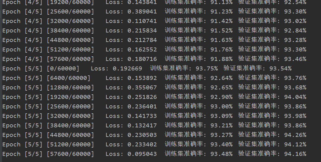
Identification results: