Welcome to "Python from zero to one", where I will share about 200 Python series articles, take you to learn and play, and see the interesting world of Python. All articles will be explained in combination with cases, codes and the author's experience. I really want to share my nearly ten years of programming experience with you. I hope it will be helpful to you. Please forgive me for the shortcomings in the article. The overall framework of Python series includes 10 basic grammars, 30 web crawlers, 10 visual analysis, 20 machine learning, 20 big data analysis, 30 image recognition, 40 artificial intelligence, 20 Python security and 10 other skills. Your attention, praise and forwarding are the greatest support for xiuzhang. Knowledge is priceless and people are affectionate. I hope we can all be happy and grow together on the road of life.
The previous article describes the data analysis part, which mainly popularizes the basic concepts of network data analysis, describes the data analysis process and related technologies, and explains in detail several third-party data analysis libraries provided by python, including Numpy, Pandas, Matplotlib, Sklearn, etc. This paper introduces the principle knowledge of regression model, including linear regression, polynomial regression and logical regression, and introduces in detail the linear regression and logistic regression algorithms of Python Sklearn machine learning library and regression analysis examples. Enter the basic article, hoping to help you.
Download address:
Previous appreciation:
Part I basic grammar
- [Python from zero to one] one Why should we learn Python and basic syntax
- [Python from zero to one] two Conditional statements, loop statements and functions based on grammar
- [Python from zero to one] three Syntax based file operation, CSV file reading and writing and object-oriented
Part II web crawler
- [Python from zero to one] four Introduction to web crawler and regular expression blog case
- [Python from zero to one] five Detailed explanation of the basic grammar of the web crawler beautiful soup
- [Python from zero to one] six Detailed explanation of the top 250 movie of BeautifulSoup crawling watercress
- [Python from zero to one] seven Web crawler Requests crawls Douban movie TOP250 and CSV storage
- [Python from zero to one] eight Basic knowledge and operation of MySQL database
- [Python from zero to one] nine Detailed explanation of Selenium basic technology of web crawler (positioning elements, common methods, keyboard and mouse operation)
- [Python from zero to one] ten Web crawler Selenium crawls online encyclopedia knowledge in ten thousand words (NLP corpus construction essential skills)
Part III data analysis and machine learning
- [Python from zero to one] eleven Introduction to Numpy, Pandas, Matplotlib and Sklearn of data analysis (1)
- [Python from zero to one] twelve Regression analysis of machine learning 10000 word summary network launch (linear regression, polynomial regression, logical regression)
The author's new "Na Zhang AI security house" will focus on Python and security technology, and mainly share articles such as Web penetration, system security, artificial intelligence, big data analysis, image recognition, malicious code detection, CVE reproduction, threat intelligence analysis, etc. Although the author is a technical white, I will ensure that every article will be written carefully. I hope these basic articles will help you and make progress with you on the Python and security road.
Supervised Learning includes classification algorithm and regression algorithm, which are defined according to the type of category label distribution. Regression algorithm is used for continuous data prediction, and classification algorithm is used for discrete distribution prediction. As one of the most important tools in statistics, regression algorithm establishes a regression equation to predict the target value and solve the regression coefficient of the regression equation.
I regression
1. What is regression
Regression was first proposed by British biostatistician Gordon and his student Pearson when studying the genetic characteristics of parents and children's height. In 1855, they described in the "regression of genetic height to the average" that "the height of children tends to be higher than the average height of their parents, but generally will not exceed the height of their parents", and put forward the concept of regression for the first time. Now regression analysis has nothing to do with this trend effect. It just refers to the mathematical method derived from Galton's work to predict the dependent variable with one or more independent variables.
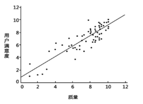
Figure 1 is a simple regression model. The X coordinate is the quality and the Y coordinate is the user satisfaction. It can be seen from the figure that the higher the quality of the product, the better the user evaluation. This can fit a straight line to predict the user satisfaction of the new product.
In the regression model, the variables we need to predict are called dependent variables, such as product quality; The variables selected to explain the changes of dependent variables are called independent variables, such as user satisfaction. The purpose of regression is to establish a regression equation to predict the target value. The whole process of regression is to find the regression coefficient of the regression equation.
In short, the simplest definition of regression is:
- Give a point set, construct a function to fit the point set, and minimize the error between the point set and the fitting function as much as possible. If the function curve is a straight line, it is called linear regression. If the curve is a cubic curve, it is called cubic multinomial regression.
2. Linear regression
Firstly, the author cites an example similar to the linear regression in the open course of machine learning at Stanford University to explain the basic knowledge and application of linear regression for your understanding. At the same time, the author strongly recommends that you learn the original Stanford open course of machine learning by Professor Andrew Ng, which will benefit you very much.
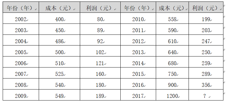
Suppose there is a data set in Table 1, which is the cost and profit data set of an enterprise. The data set from 2002 to 2016 in the data set is called the training set. There are 15 sample data in the whole training set. The focus is on two variables: cost and profit. Cost is an input variable or a feature, and profit is an output variable or target variable. The whole regression model is shown in Figure 2.
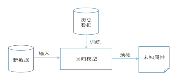
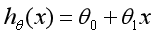
The model is now established. x represents the enterprise cost, Y represents the enterprise profit, and h (Hypothesis) represents the function that maps the input variable to the output variable y. The linear regression (univariate linear regression) formula corresponding to a dependent variable is as follows:
Then, the problem to be solved now is how to solve the two parameters and. Our idea is to select the parameters and make the function as close to the y value as possible. Here, we propose to find the square error function of the training set (x,y) or the least square method.
In the regression equation, the method of minimizing the sum of squares of errors is the best method to find the characteristic corresponding regression coefficient. Error refers to the difference between the predicted y value and the real y value. The simple accumulation of errors will make the positive difference and negative difference offset each other. The square error (least square method) adopted is as follows:

Mathematically, the solution process is transformed into finding a set of values to minimize the above formula. The most common solution method is the Gradient Descent method. According to the square error, the loss function of the linear regression model is defined as, and the formula is as follows:
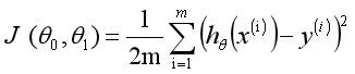
The fitting solution process can be realized by selecting appropriate parameters to minimize min. Through the above example, we can define the linear regression model as follows: estimate the function h according to the coordinates of sample x and y, and seek the approximate functional relationship between variables. The formula is as follows:
Where n represents the number of features and the ith special value of each training sample. When there is only one dependent variable x, it is called univariate linear regression, similar to; When there are multiple dependent variables, it becomes multiple linear regression. Our purpose is to minimize the sample data set, so as to best fit the sample data set and better predict the new data.
Polynomial regression or logistic regression will be introduced later.
II Linear regression analysis
Linear regression is one of the basic algorithms in data mining. Its core idea is to solve a set of equations between dependent variables and independent variables to obtain the regression function. At the same time, the error term is usually calculated by the least square method. Linear will be called in the Sklaern machine learning package commonly used in this book_ The LinearRegression class of model subclass performs linear regression model calculation.
1.LinearRegression
Linear regression model in sklearn linear_ Under the model subclass, it mainly calls the fit(x,y) function to train the model, where x is the attribute of the data and Y is the type. The code of the regression model referenced in sklearn is as follows:
from sklearn import linear_model          #Import linear model
regr = linear_model.LinearRegression()    #Using linear regression
print(regr)
The output function is constructed as follows:
LinearRegression(copy_X=True,
		fit_intercept=True,
        n_jobs=1,
        normalize=False)
The parameters are described as follows:
- copy_ 10: Boolean, default to True. Whether to copy X. if False is selected, the original data will be overwritten directly, that is, after centralization and standardization, the new data will be overwritten on the original data.
- fit_intercept: Boolean; the default value is True. Whether to centralize the training data. If True, it indicates that the input training data has been centralized. If False, the input data has been centralized, and the subsequent processes will not be centralized.
- n_jobs: integer type; the default value is 1. The number of tasks set during calculation. If set to - 1, all CPU s are used. This parameter can accelerate the problem that the number of targets is greater than 1 and the scale is large enough.
- normalize: Boolean; the default is False. Whether the data is standardized.
LinearRegression class mainly includes the following methods:

- fit(X,y[,n_jobs])
Train the training sets X and y, analyze the model parameters and fill the data set. Where x is the feature and Y is the tag or class attribute. - predict(X)
The trained estimator or model is used to predict the input x data set, and the returned result is the predicted value. Data set X is usually divided into training set and test set. - decision_function(X)
The trained estimator or model is used to predict the data set X. The difference between it and predict(X) is that this method includes the type check of input data and whether the current object has a coef_ Property, more secure. - score(X, y[,]samples_weight)
Returns the score of prediction effect with X as samples and y as target. - get_params([deep])
Gets the parameters of the Estimator. - **set_params(params)
Set the parameters of the Estimator. - coef_
Store the regression coefficients of linear regression model. - intercept_
Store the regression intercept of linear regression model.
Now the linear regression experiment is carried out on the previous enterprise cost and profit data set. The complete code is as follows:
# -*- coding: utf-8 -*-
# By:Eastmount CSDN 2021-07-03
from sklearn import linear_model #Import linear model
import matplotlib.pyplot as plt
import numpy as np
#X represents enterprise cost and Y represents enterprise profit
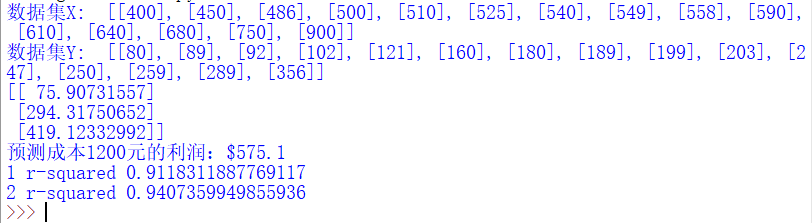
X = [[400], [450], [486], [500], [510], [525], [540], [549], [558], [590], [610], [640], [680], [750], [900]]
Y = [[80], [89], [92], [102], [121], [160], [180], [189], [199], [203], [247], [250], [259], [289], [356]]
print('data set X: ', X)
print('data set Y: ', Y)
#Regression training
clf = linear_model.LinearRegression()
clf.fit(X, Y)
#Prediction results
X2 = [[400], [750], [950]]
Y2 = clf.predict(X2)
print(Y2)
res = clf.predict(np.array([1200]).reshape(-1, 1))[0]
print('Profit with predicted cost of 1200 yuan: $%.1f' % res)
#Draw linear regression graph
plt.plot(X, Y, 'ks') #Draw training data distribution point map
plt.plot(X2, Y2, 'g-') #Draw forecast dataset lines
plt.show()
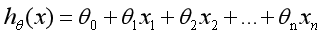
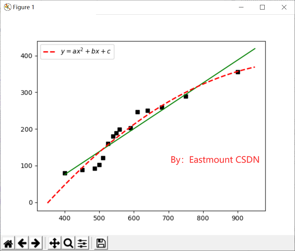
Call the LinearRegression() regression function in the sklearn package, load fit(X,Y) into the data set for training, then predict(X2) the profit of data set X2, draw the prediction result into a straight line, and draw the (X,Y) data set into a scatter diagram, as shown in Figure 3.
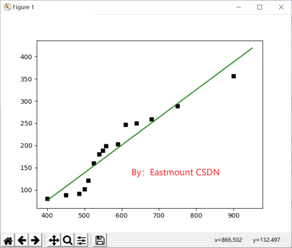
At the same time, the code is called to predict that the enterprise cost in 2017 is 1200 yuan and the profit is 575.1 yuan. Note that the regression coefficients of the linear model are saved in the coef_ Variable, the intercept is saved in intercept_ Variable. clf.score(X, Y) is a scoring function that returns a score less than 1. The code of scoring process is as follows:
print('coefficient', clf.coef_)
print('intercept', clf.intercept_)
print('Scoring function', clf.score(X, Y))

'''
coefficient [[ 0.62402912]]
intercept [-173.70433885]
Scoring function 0.911831188777
'''
The regression function corresponding to the straight line is: y = 0.62402912 * x - 173.70433885, then the predicted profit value of X2[1]=400 is 75.9, while the cost in X1 is 400 yuan, the corresponding real profit is 80 yuan, and the prediction is basically accurate.
2. linear regression predicts diabetes mellitus.
(1). Diabetes dataset
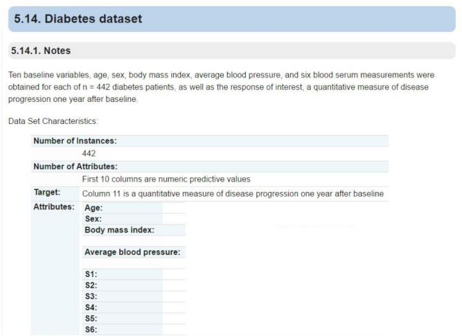
The Sklearn machine learning package provides the Diabetes Dataset (dataset), which contains 442 rows of data and 10 eigenvalues, namely: age (Age), gender (Sex), body mass index (Body mass index), mean blood pressure (Average Blood Pressure), and disease progression index after one year. The predictive index is Target, which represents the quantitative index of disease one year later. The description of the original website is shown in Figure 4:
The following code is used for simple call and data scale test.
# -*- coding: utf-8 -*-
# By:Eastmount CSDN 2021-07-03
from sklearn import datasets
diabetes = datasets.load_diabetes()                           #Load data
print(diabetes.data)                                          #data
print(diabetes.target)                                        #Class standard
print('Total number of rows: ', len(diabetes.data), len(diabetes.target))
print('Characteristic number: ', len(diabetes.data[0]))                      #Data set dimension per row
print('data type: ', diabetes.data.shape)
print(type(diabetes.data), type(diabetes.target))
Call load_ The diabetes () function loads the diabetes dataset and outputs its data data and class target. The total number of output lines is 442, the total number of features is 10, and the type is (442L, 10L). Its output is as follows:
[[ 0.03807591  0.05068012  0.06169621 ..., -0.00259226  0.01990842
  -0.01764613]
 [-0.00188202 -0.04464164 -0.05147406 ..., -0.03949338 -0.06832974
  -0.09220405]
  ...
 [-0.04547248 -0.04464164 -0.0730303  ..., -0.03949338 -0.00421986
   0.00306441]]
[ 151.   75.  141.  206.  135.   97.  138.   63.  110.  310.  101.
  ...
64.   48.  178.  104.  132.  220.   57.]
Total number of rows:  442 442
Characteristic number:  10
data type:  (442L, 10L)
<type 'numpy.ndarray'> <type 'numpy.ndarray'>
(2). code implementation
Now we divide the diabetes dataset into training set and test set. The whole dataset has 442 rows. We take the first 422 rows of data to train the linear regression model, and the 20 row data are used to predict. The code of the forecast data is diabetes_x_temp[-20:] means that the value is taken from the last 20 lines to the end of the array. There are 20 values in total.
There are 10 eigenvalues in the whole data set. In order to facilitate visual drawing, we only obtain one of them for experiments, which can also draw graphics. In real analysis, graphics are usually drawn after dimension reduction. Here, the third feature is obtained, and the corresponding code is: diabetes_x_temp = diabetes.data[:, np.newaxis, 2]. The complete code is as follows:
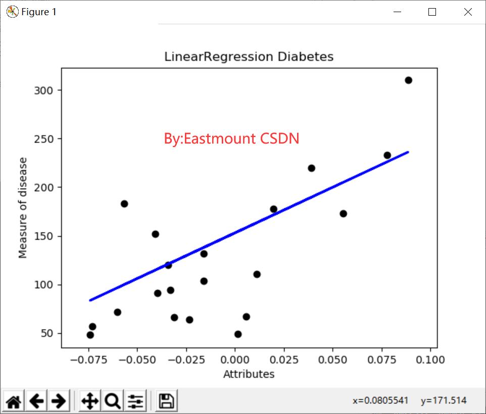
# -*- coding: utf-8 -*-
# By:Eastmount CSDN 2021-07-03
from sklearn import datasets
import matplotlib.pyplot as plt
from sklearn import linear_model
import numpy as np

#Data set partition
diabetes = datasets.load_diabetes()                #Load data
diabetes_x_temp = diabetes.data[:, np.newaxis, 2]  #Get one of the features
diabetes_x_train = diabetes_x_temp[:-20]           #training sample
diabetes_x_test = diabetes_x_temp[-20:]            #20 lines after test sample
diabetes_y_train = diabetes.target[:-20]           #Training mark
diabetes_y_test = diabetes.target[-20:]            #Prediction comparison mark

#Regression training and prediction
clf = linear_model.LinearRegression()
clf.fit(diabetes_x_train, diabetes_y_train)        #Training data set
pre = clf.predict(diabetes_x_test)

#mapping
plt.title(u'LinearRegression Diabetes')            #title
plt.xlabel(u'Attributes')                          #x-coordinate
plt.ylabel(u'Measure of disease')                  #y-axis coordinates
plt.scatter(diabetes_x_test, diabetes_y_test, color = 'black')  #Scatter diagram
plt.plot(diabetes_x_test, pre, color='blue', linewidth = 2)     #Prediction line
plt.show()
The output result is shown in Figure 5. Each point represents the real value, and the straight line represents the predicted result.
(3). Code optimization
The following code adds several optimization measures, including the calculation of slope and intercept, the visual drawing, the distance line from scattered points to linear equation, and the pixel code for saving pictures, etc. These optimizations help us better analyze real data sets.
# -*- coding: utf-8 -*-
# By:Eastmount CSDN 2021-07-03
from sklearn import datasets
import numpy as np
from sklearn import linear_model
import matplotlib.pyplot as plt

#Step 1 data set division
d = datasets.load_diabetes()  #Data 10 * 442
x = d.data
x_one = x[:,np.newaxis, 2]    #Get the third column data of a feature
y = d.target                  #Get correct results
x_train = x_one[:-42]         #Training set X [0:400]
x_test = x_one[-42:]          #Prediction set X [401:442]
y_train = y[:-42]             #Training set Y [0:400]
y_test = y[-42:]              #Prediction set Y [401:442]

#The second step is the realization of linear regression
clf = linear_model.LinearRegression()
print(clf)
clf.fit(x_train, y_train)
pre = clf.predict(x_test)
print('Prediction results', pre)
print('Real results', y_test)

#Step 3 evaluation results
cost = np.mean(y_test-pre)**2   #Power 2
print('Square sum calculation:', cost)
print('coefficient', clf.coef_)
print('intercept', clf.intercept_)
print('variance', clf.score(x_test, y_test))

#Step 4 drawing
plt.plot(x_test, y_test, 'k.')      #Scatter diagram
plt.plot(x_test, pre, 'g-')        #Prediction regression line
#Draw point to line distance
for idx, m in enumerate(x_test):
    plt.plot([m, m],[y_test[idx], pre[idx]], 'r-')

plt.savefig('blog12-01.png', dpi=300) #Save picture
plt.show()
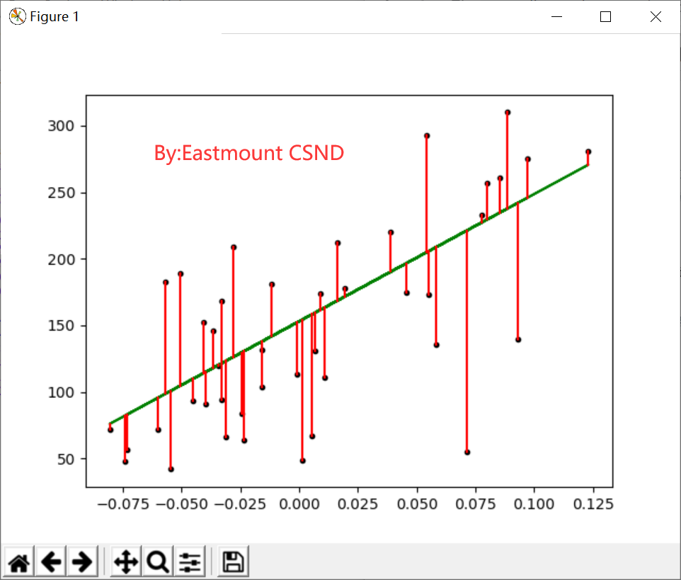
The drawing is shown in Figure 6.
The output results are as follows:
LinearRegression(copy_X=True, fit_intercept=True, n_jobs=1, normalize=False)
Prediction results [ 196.51241167  109.98667708  121.31742804  245.95568858  204.75295782
  270.67732703   75.99442421  241.8354155   104.83633574  141.91879342
  126.46776938  208.8732309   234.62493762  152.21947611  159.42995399
  161.49009053  229.47459628  221.23405012  129.55797419  100.71606266
  118.22722323  168.70056841  227.41445974  115.13701842  163.55022706
  114.10695016  120.28735977  158.39988572  237.71514243  121.31742804
   98.65592612  123.37756458  205.78302609   95.56572131  154.27961264
  130.58804246   82.17483382  171.79077322  137.79852034  137.79852034
  190.33200206   83.20490209]
Real results [ 175.   93.  168.  275.  293.  281.   72.  140.  189.  181.  209.  136.
  261.  113.  131.  174.  257.   55.   84.   42.  146.  212.  233.   91.
  111.  152.  120.   67.  310.   94.  183.   66.  173.   72.   49.   64.
   48.  178.  104.  132.  220.   57.]

Square sum calculation: 83.192340827
 coefficient [ 955.70303385]
Intercept 153.000183957
 Variance 0.427204267067
Where cost = NP Mean (y_test pre) * * 2 represents the sum of squares between the calculated prediction result and the real result, which is 83.192340827. According to the coefficient and intercept, the equation is: y = 955.70303385 * x + 153.000183957.
III Polynomial regression analysis
1. Basic concepts
Linear regression studies the regression between a target variable and an independent variable, but sometimes in many practical problems, the independent variable affecting the target variable is often more than one, but more than one. For example, the wool yield of sheep is affected by multiple variables such as sheep weight, chest circumference and body length, Therefore, it is necessary to design a regression analysis between a target variable and multiple independent variables, that is, multiple regression analysis. Since linear regression is not applicable to all data, we need to establish curves to adapt to our data. Many curve relationships in the real world are realized by adding polynomials, such as a quadratic function model:
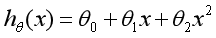
Or a cubic function model:

The figures drawn by us for these two models are as follows:
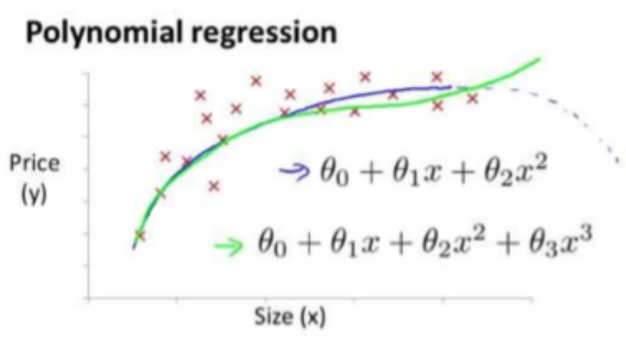
Polynomial Regression is a Polynomial Regression analysis method to study the relationship between a dependent variable and one or more independent variables. If there is only one independent variable, it is called univariate Polynomial Regression; If there are multiple independent variables, it is called multivariate Polynomial Regression. In univariate regression analysis, if the relationship between dependent variable y and independent variable x is nonlinear, but no appropriate function curve can be found to fit, univariate Polynomial Regression can be used. Section 17.3 mainly explains the Polynomial Regression analysis of univariate multiple times. The univariate m-degree polynomial equation is as follows:
The process of solving the equation is expected to be learned by readers. Next, the author mainly explains how Python code realizes polynomial regression analysis.
2.PolynomialFeatures
Python polynomial regression needs to import sklearn The PolynomialFeatures class in the preprocessing subclass is implemented. The function prototype corresponding to PolynomialFeatures is as follows:
class sklearn.preprocessing.PolynomialFeatures(degree=2,
		interaction_only=False,
		include_bias=True)
PolynomialFeatures class is explained on the Sklearn official website: models or classes that specifically generate polynomials, and polynomials contain interactive feature sets. There are three parameters in total. degree represents the polynomial order, and the general default value is 2; interaction_only if the value is true (False by default), interactive feature sets will be generated; include_bias indicates whether the deviation column is included.
PolynomialFeatures class establishes an arithmetic sequence matrix by instantiating a polynomial, then carries out training and prediction, finally draws relevant graphics, and then compares it with the previous univariate linear regression analysis.
3. Polynomial regression to predict cost and profit
This section mainly explains the example of polynomial regression analysis. The data set analyzed is the enterprise cost and profit data set provided in table 17.1. The complete code and detailed notes for the comparison of linear regression and polynomial regression analysis are directly given below.
# -*- coding: utf-8 -*-
# By:Eastmount CSDN 2021-07-03
from sklearn.linear_model import LinearRegression
from sklearn.preprocessing import PolynomialFeatures
import matplotlib.pyplot as plt
import numpy as np

#X represents enterprise cost and Y represents enterprise profit
X = [[400], [450], [486], [500], [510], [525], [540], [549], [558], [590], [610], [640], [680], [750], [900]]
Y = [[80], [89], [92], [102], [121], [160], [180], [189], [199], [203], [247], [250], [259], [289], [356]]
print('data set X: ', X)
print('data set Y: ', Y)

#The first step is linear regression analysis
clf = LinearRegression()
clf.fit(X, Y)
X2 = [[400], [750], [950]]
Y2 = clf.predict(X2)
print(Y2)
res = clf.predict(np.array([1200]).reshape(-1, 1))[0]
print('Profit with predicted cost of 1200 yuan: $%.1f' % res)
plt.plot(X, Y, 'ks')    #Draw training data distribution point map
plt.plot(X2, Y2, 'g-')  #Draw forecast dataset lines

#The second step is polynomial regression analysis
xx = np.linspace(350,950,100) #350 to 950 equal difference series
quadratic_featurizer = PolynomialFeatures(degree = 2) #Instantiate a quadratic polynomial
x_train_quadratic = quadratic_featurizer.fit_transform(X) #Transform with quadratic polynomial x
X_test_quadratic = quadratic_featurizer.transform(X2)
regressor_quadratic = LinearRegression()
regressor_quadratic.fit(x_train_quadratic, Y)

#The polynomial characteristic example of trained X value is applied to a series of points to form a matrix
xx_quadratic = quadratic_featurizer.transform(xx.reshape(xx.shape[0], 1))
plt.plot(xx, regressor_quadratic.predict(xx_quadratic), "r--",
         label="$y = ax^2 + bx + c$",linewidth=2)
plt.legend()
plt.show()
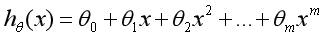
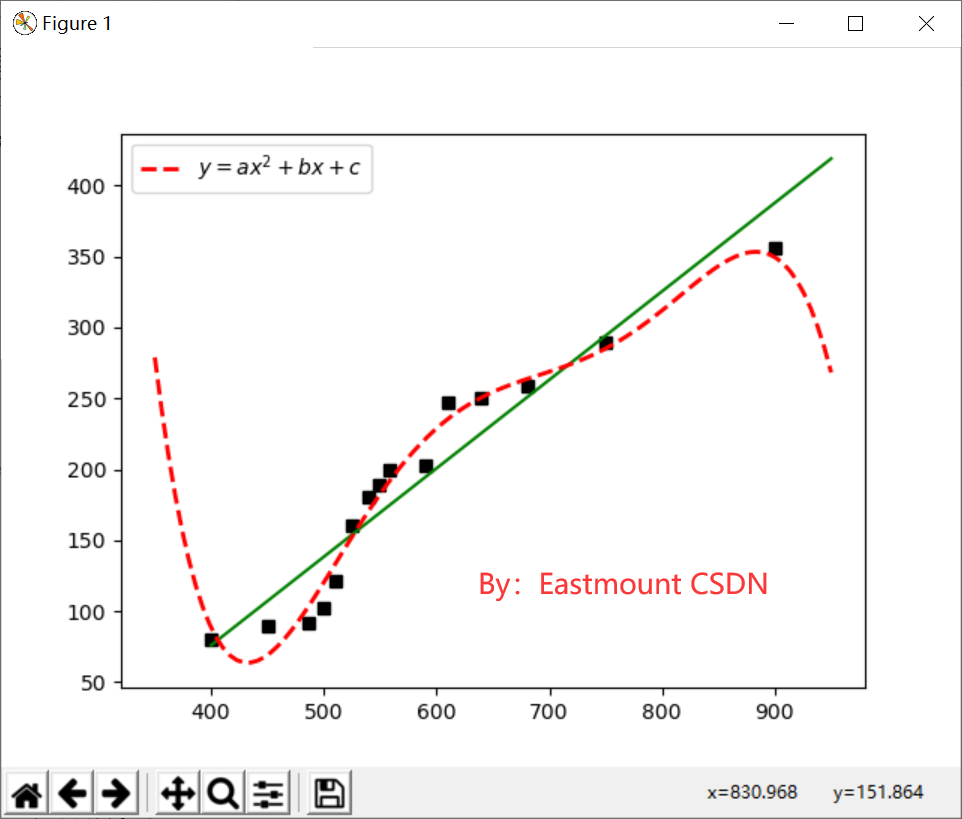
The output graph is shown in the figure below, in which the black scatter diagram represents the real relationship between enterprise cost and profit, the green straight line is a univariate linear regression equation, and the red virtual curve is a quadratic polynomial equation. It is closer to the real scatter diagram.
Here, we use R-square to evaluate the effect of polynomial regression prediction. R-square is also called Coefficient of Determination, which represents the degree of fitting of the model to real data. There are several methods to calculate the R-square. In univariate linear regression, the R-square is equal to the square of Pearson Product Moment Correlation Coefficient. The R-square calculated by this method is a positive number between 0 and 1. The other is the method provided by Sklearn library to calculate the R-square. The calculation code of Party R is as follows:
print('1 r-squared', clf.score(X, Y))
print('2 r-squared', regressor_quadratic.score(x_train_quadratic, Y))
The output is as follows:
('1 r-squared', 0.9118311887769025)
('2 r-squared', 0.94073599498559335)
The R-square value of univariate linear regression is 0.9118 and that of polynomial regression is 0.9407, indicating that more than 94% of the prices in the data set can be explained by the model. Finally, the fitting process of five terms is supplemented, and only the core code is given below.
# -*- coding: utf-8 -*-
# By:Eastmount CSDN 2021-07-03
from sklearn.linear_model import LinearRegression
from sklearn.preprocessing import PolynomialFeatures
import matplotlib.pyplot as plt
import numpy as np

#X represents enterprise cost and Y represents enterprise profit
X = [[400], [450], [486], [500], [510], [525], [540], [549], [558], [590], [610], [640], [680], [750], [900]]
Y = [[80], [89], [92], [102], [121], [160], [180], [189], [199], [203], [247], [250], [259], [289], [356]]
print('data set X: ', X)
print('data set Y: ', Y)

#The first step is linear regression analysis
clf = LinearRegression()
clf.fit(X, Y)
X2 = [[400], [750], [950]]
Y2 = clf.predict(X2)
print(Y2)
res = clf.predict(np.array([1200]).reshape(-1, 1))[0]
print('Profit with predicted cost of 1200 yuan: $%.1f' % res)
plt.plot(X, Y, 'ks')    #Draw training data distribution point map
plt.plot(X2, Y2, 'g-')  #Draw forecast dataset lines

#The second step is polynomial regression analysis
xx = np.linspace(350,950,100)
quadratic_featurizer = PolynomialFeatures(degree = 5)
x_train_quadratic = quadratic_featurizer.fit_transform(X)
X_test_quadratic = quadratic_featurizer.transform(X2)
regressor_quadratic = LinearRegression()
regressor_quadratic.fit(x_train_quadratic, Y)
#The polynomial characteristic example of trained X value is applied to a series of points to form a matrix
xx_quadratic = quadratic_featurizer.transform(xx.reshape(xx.shape[0], 1))
plt.plot(xx, regressor_quadratic.predict(xx_quadratic), "r--",
         label="$y = ax^2 + bx + c$",linewidth=2)
plt.legend()
plt.show()
print('1 r-squared', clf.score(X, Y))
print('5 r-squared', regressor_quadratic.score(x_train_quadratic, Y))

# ('1 r-squared', 0.9118311887769025)
# ('5 r-squared', 0.98087802460869788)
The output is as follows. The red dotted line is a quintic polynomial curve, which is closer to the distribution of the real data set, while the green straight line is a univariate linear regression equation. Obviously, the fitting result of the linear equation is worse than that of the quintic polynomial curve. At the same time, the R-square value of quintic polynomial curve is 98.08%, which can accurately predict the data trend.
Finally, it is suggested that the order of polynomial regression should not be too high, otherwise over fitting will occur.
IV logistic regression
1. Basic principle
In the regression model described above, the dependent variables are numerical interval variables, and the established model describes the linear relationship or polynomial curve relationship between the expectation of the dependent variable and the independent variable. For example, common linear regression models:

In the analysis of practical problems by regression model, the variables studied are often not all interval variables, but sequential variables or attribute variables, such as binomial distribution problem. By analyzing age, gender, body mass index, mean blood pressure, disease index and other indicators, we can judge whether a person is changing diabetes. Y=0 means that she is not sick. Y=1 means sickness. The response variable here is a two point (0 or 1) distribution variable. It can not predict the dependent variable Y (Y can only take 0 or 1) with the continuous value of h function.
In short, linear regression or polynomial regression models usually deal with the problem that the dependent variable is a continuous variable. If the dependent variable is a qualitative variable, the linear regression model is no longer applicable. At this time, it needs to be solved by logical regression model.
Logistic Regression is used to deal with the regression problem in which the dependent variable is classified variable. The common problem is binary classification or binomial distribution. It can also deal with multi classification problems. In fact, it belongs to a classification method.
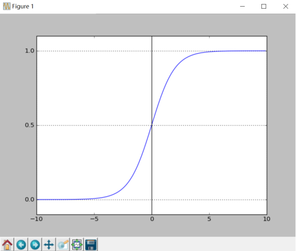
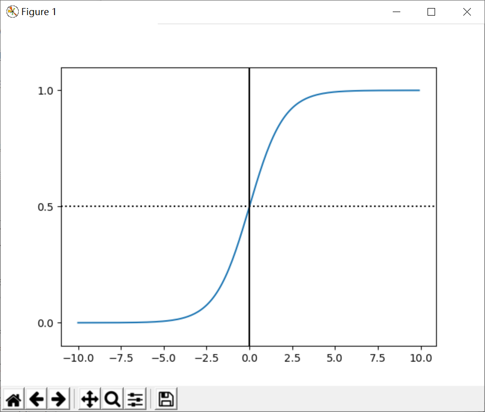
The graph of the relationship between the probability and independent variables of the binary classification problem is often an S-shaped curve, as shown in figure 17.10, which is realized by Sigmoid function. Here we define this function as follows:
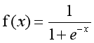
The definition field of the function is all real numbers, the value field is between [0,1], and the corresponding result of the x-axis at point 0 is 0.5. When the value of X is large enough, it can be regarded as two types of problems: 0 or 1. If it is greater than 0.5, it can be regarded as a class 1 problem. On the contrary, it is a Class 0 problem, and if it is just 0.5, it can be divided into class 0 or class 1. For 0-1 variables, the probability distribution formula of y=1 is defined as follows:
The probability distribution formula of y=0 is defined as follows:

The expected value formula of discrete random variables is as follows:
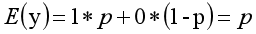
The linear model is adopted for analysis, and the formula transformation is as follows:

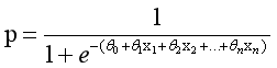
In practical application, probability p and dependent variables are often nonlinear. In order to solve this kind of problem, we introduce logit transformation, so that there is a linear correlation between logit § and independent variables. The logical regression model is defined as follows:

Through derivation, the probability P transformation is as follows, which is consistent with the Sigmoid function and reflects the nonlinear relationship between probability P and dependent variables. Taking 0.5 as the limit, when p is predicted to be greater than 0.5, we judge that y is more likely to be 1 at this time, otherwise y is 0.
After obtaining the required Sigmoid function, we only need to fit the n parameters in the formula like the previous linear regression θ Just. The following is to draw the Sigmoid curve, and the output is shown in Figure 10.
# -*- coding: utf-8 -*-
# By:Eastmount CSDN 2021-07-03
import matplotlib.pyplot as plt
import numpy as np

def Sigmoid(x):
    return 1.0 / (1.0 + np.exp(-x))

x= np.arange(-10, 10, 0.1)
h = Sigmoid(x)                #Sigmoid function
plt.plot(x, h)
plt.axvline(0.0, color='k')   #Add a vertical line on the coordinate axis (position 0)
plt.axhspan(0.0, 1.0, facecolor='1.0', alpha=1.0, ls='dotted')
plt.axhline(y=0.5, ls='dotted', color='k')
plt.yticks([0.0, 0.5, 1.0])  #y-axis scale
plt.ylim(-0.1, 1.1)          #y-axis range
plt.show()
Due to the limited space, the loss function J function is constructed by logistic regression to solve the minimum J function and regression parameters θ The method is not in narration. The principle is the same as that introduced earlier. Please go on and study it in depth.
2.LogisticRegression
Logistic regression model in sklearn linear_ Under the model subclass, the steps of calling sklearn logistic regression algorithm are relatively simple, that is:
- Import the model. Call the logistic regression() function.
- fit() training. Call the method of fit(x,y) to train the model, where x is the attribute of the data and Y is the type.
- predict(). The trained model is used to predict the data set and return the prediction results.
The code is as follows:
# -*- coding: utf-8 -*-
# By:Eastmount CSDN 2021-07-03
from sklearn.linear_model import LogisticRegression  #Import logistic regression model
clf = LogisticRegression()
print(clf)
clf.fit(train_feature,label)
predict['label'] = clf.predict(predict_feature)
The output function is constructed as follows:
LogisticRegression(C=1.0, class_weight=None, dual=False, fit_intercept=True,
          intercept_scaling=1, max_iter=100, multi_class='ovr', n_jobs=1,
          penalty='l2', random_state=None, solver='liblinear', tol=0.0001,
          verbose=0, warm_start=False)
Only two parameters are introduced here: the parameter penalty represents a penalty item, including two optional values L1 and L2. L1 represents the sum of the absolute values of each element in the vector, which is often used for feature selection; L2 represents the sum of squares of each element in the vector and then the root sign. When more features need to be selected, L2 parameter is used to make them close to 0. The objective function constraint condition of C value is: S.T. | w| 1 < C, the default value is 0, and the smaller the C value, the greater the regularization intensity.
3. Regression analysis example of iris data set
Next, the iris data set will be analyzed combined with the logistic regression model of scikit learn official website. Because the data classification label is divided into three categories (category 0, category 1 and category 2), it belongs to three classification problems, so it can be analyzed by logistic regression model.
(1). Iris dataset
In the Sklearn machine learning package, various data sets are integrated, including the previous diabetes dataset. The iris dataset (Iris) is introduced here, and it is also a very common dataset. The data set contains 4 characteristic variables and 1 category variable, with a total of 150 samples. Among them, four features are sepal length and width, petal length and width. One category variable is the classification of marked iris, which includes three cases, namely iris setosa, iris versicolor and iris Virginia. The detailed introduction of iris data set is shown in Table 2:
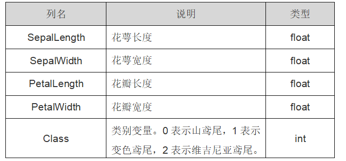
Class variable. 0 represents mountain iris, 1 represents discolored iris, and 2 represents Virginia iris. int
There are two attributes in iris data,iris.target. Data is a matrix. Each column represents the length and width of sepals or petals. There are four columns in total. Each row represents a measured iris plant. A total of 150 records, i.e. 150 iris samples, were sampled.
from sklearn.datasets import load_iris   #Import dataset iris
iris = load_iris()  #Load dataset
print(iris.data)
The output is as follows:
[[ 5.1  3.5  1.4  0.2]
 [ 4.9  3.   1.4  0.2]
 [ 4.7  3.2  1.3  0.2]
 [ 4.6  3.1  1.5  0.2]
 ....
 [ 6.7  3.   5.2  2.3]
 [ 6.3  2.5  5.   1.9]
 [ 6.5  3.   5.2  2. ]
 [ 6.2  3.4  5.4  2.3]
 [ 5.9  3.   5.1  1.8]]
target is an array that stores which kind of iris plant the sample corresponding to each row of data belongs to, either mountain iris (value 0), color changing iris (value 1), or Virginia iris (value 2). The length of the array is 150.
print(iris.target)           #Output real label
print(len(iris.target))      #150 samples, 4 features per sample
print(iris.data.shape)

[0 0 0 0 0 0 0 0 0 0 0 0 0 0 0 0 0 0 0 0 0 0 0 0 0 0 0 0 0 0 0 0 0 0 0 0 0
 0 0 0 0 0 0 0 0 0 0 0 0 0 1 1 1 1 1 1 1 1 1 1 1 1 1 1 1 1 1 1 1 1 1 1 1 1
 1 1 1 1 1 1 1 1 1 1 1 1 1 1 1 1 1 1 1 1 1 1 1 1 1 1 2 2 2 2 2 2 2 2 2 2 2
 2 2 2 2 2 2 2 2 2 2 2 2 2 2 2 2 2 2 2 2 2 2 2 2 2 2 2 2 2 2 2 2 2 2 2 2 2
 2 2]
150
(150L, 4L)
From the output results, we can see that the class marks are divided into three categories: the first 50 class marks are 0, the middle 50 class marks are 1, and the back is 2. The code for analyzing this data set using logistic regression is described in detail below.
(2). Scatter plot
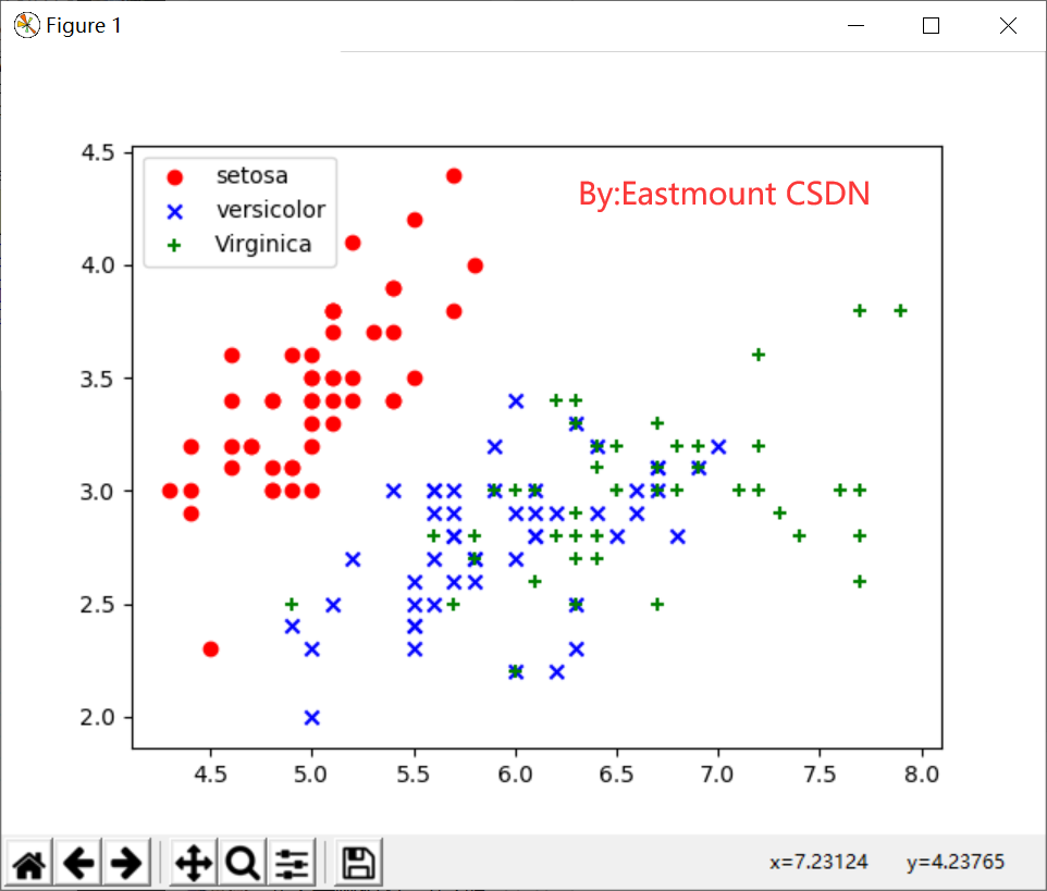
After loading the iris data set (data and label target), we need to obtain two columns of data or two features, and then call the scatter() function to draw the scatter diagram. The core code for obtaining a feature is: X = [x[0] for x in DD], and assign the obtained value to the X variable. The complete code is as follows:
# -*- coding: utf-8 -*-
# By:Eastmount CSDN 2021-07-03
import matplotlib.pyplot as plt
import numpy as np
from sklearn.datasets import load_iris    #Import dataset iris

#Load dataset
iris = load_iris()
print(iris.data)           #Output dataset
print(iris.target)         #Output real label

#Get two column dataset
DD = iris.data
X = [x[0] for x in DD]
print(X)
Y = [x[1] for x in DD]
print(Y)

#plt.scatter(X, Y, c=iris.target, marker='x')
plt.scatter(X[:50], Y[:50], color='red', marker='o', label='setosa') #First 50 samples
plt.scatter(X[50:100], Y[50:100], color='blue', marker='x', label='versicolor') #Middle 50
plt.scatter(X[100:], Y[100:],color='green', marker='+', label='Virginica') #Last 50 samples
plt.legend(loc=2) #top left corner
plt.show()
The output is shown in Figure 11:
(3). Linear regression analysis
The following code first obtains the first two columns of iris data set, and then calls the linear regression model in Sklearn library for analysis. The complete code is shown in the file.
# -*- coding: utf-8 -*-
# By:Eastmount CSDN 2021-07-03
#Step 1 import dataset
from sklearn.datasets import load_iris
hua = load_iris()
#Gets the length and width of the petals
x = [n[0] for n in hua.data]
y = [n[1] for n in hua.data]
import numpy as np #Convert to array
x = np.array(x).reshape(len(x),1)
y = np.array(y).reshape(len(y),1)
#The second step is linear regression analysis
from sklearn.linear_model import LinearRegression
clf = LinearRegression()
clf.fit(x,y)
pre = clf.predict(x)
print(pre)
#Step 3 draw
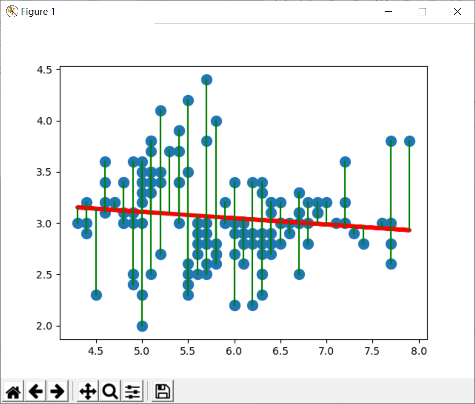
import matplotlib.pyplot as plt
plt.scatter(x,y,s=100)
plt.plot(x,pre,"r-",linewidth=4)
for idx, m in enumerate(x):
plt.plot([m,m],[y[idx],pre[idx]], 'g-')
plt.show()
The output graph is shown in Figure 12, and you can see the distance from all scatter points to the fitted univariate linear equation.
(4). Logistic regression analysis of iris
After explaining the linear regression analysis, what is the result of logistic regression analysis? Let's start. It can be seen from the scatter diagram (FIG. 11) that the data set is linearly separable and is divided into three categories, corresponding to three types of iris respectively. Next, it is analyzed and predicted by logistic regression.
Previously, X=[x[0] for x in DD] is used to obtain the first column of data, and Y=[x[1] for x in DD] is used to obtain the second column of data. Here, another method is used, iris Data [:,: 2] obtain two columns of data or two features. The complete code is as follows:
# -*- coding: utf-8 -*-
# By:Eastmount CSDN 2021-07-03
import matplotlib.pyplot as plt
import numpy as np
from sklearn.datasets import load_iris
from sklearn.linear_model import LogisticRegression
#Load dataset
iris = load_iris()
X = X = iris.data[:, :2] #Get two column dataset
Y = iris.target
#Logistic regression model
lr = LogisticRegression(C=1e5)
lr.fit(X,Y)
#The meshgrid function generates two grid matrices
h = .02
x_min, x_max = X[:, 0].min() - .5, X[:, 0].max() + .5
y_min, y_max = X[:, 1].min() - .5, X[:, 1].max() + .5
xx, yy = np.meshgrid(np.arange(x_min, x_max, h), np.arange(y_min, y_max, h))
#The pcolormesh function draws the two grid matrices XX and YY and the corresponding prediction result Z on the picture
Z = lr.predict(np.c_[xx.ravel(), yy.ravel()])
Z = Z.reshape(xx.shape)
plt.figure(1, figsize=(8,6))
plt.pcolormesh(xx, yy, Z, cmap=plt.cm.Paired)
#Scatter plot
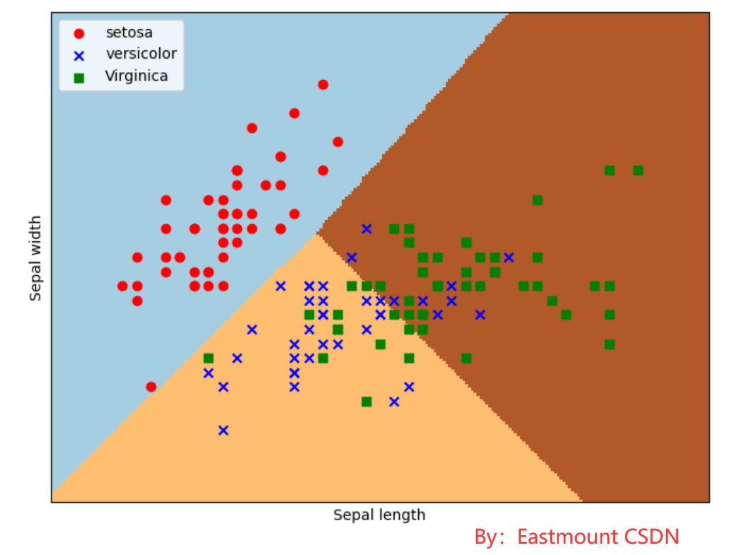
plt.scatter(X[:50,0], X[:50,1], color='red',marker='o', label='setosa')
plt.scatter(X[50:100,0], X[50:100,1], color='blue', marker='x', label='versicolor')
plt.scatter(X[100:,0], X[100:,1], color='green', marker='s', label='Virginica')
plt.xlabel('Sepal length')
plt.ylabel('Sepal width')
plt.xlim(xx.min(), xx.max())
plt.ylim(yy.min(), yy.max())
plt.xticks(())
plt.yticks(())
plt.legend(loc=2)
plt.show()
The output is shown in Figure 13. After logistic regression, it is divided into three regions. The upper left corner is red dots, corresponding to setosa iris; The upper right corner is a green square, corresponding to virginica iris; The middle lower part is a blue star, corresponding to versicolor iris. The scatter diagram shows the real flower types of each data point, and the divided three areas are the flower types predicted by the data points. The predicted classification results are basically consistent with the real results of the training data, and some iris flowers cross.
Next, the author explains the code after importing the dataset in detail.
- lr = LogisticRegression(C=1e5)
Initialize the logistic regression model, and C=1e5 represents the objective function. - lr.fit(X,Y)
Call the logistic regression model for training. Parameter X is the data feature and parameter Y is the data class standard. - x_min, x_max = X[:, 0].min() - .5, X[:, 0].max() + .5
- y_min, y_max = X[:, 1].min() - .5, X[:, 1].max() + .5
- xx, yy = np.meshgrid(np.arange(x_min, x_max, h), np.arange(y_min, y_max, h))
Obtain two columns of data of iris data set, corresponding to calyx length and calyx width. The coordinates of each point are (x,y). First take the minimum value, maximum value and step h (set to 0.02) of the first column (length) of the X-two-dimensional array to generate the array, then take the minimum value, maximum value and step h of the second column (width) of the X-two-dimensional array to generate the array, and finally use the meshgrid function to generate two grid matrices xx and yy, as shown below:
[[ 3.8   3.82  3.84 ...,  8.36  8.38  8.4 ]
 [ 3.8   3.82  3.84 ...,  8.36  8.38  8.4 ]
 ...,
 [ 3.8   3.82  3.84 ...,  8.36  8.38  8.4 ]
 [ 3.8   3.82  3.84 ...,  8.36  8.38  8.4 ]]
[[ 1.5   1.5   1.5  ...,  1.5   1.5   1.5 ]
 [ 1.52  1.52  1.52 ...,  1.52  1.52  1.52]
 ...,
 [ 4.88  4.88  4.88 ...,  4.88  4.88  4.88]
 [ 4.9   4.9   4.9  ...,  4.9   4.9   4.9 ]]
- Z = lr.predict(np.c_[xx.ravel(), yy.ravel()])
Call the travel() function to convert the two matrices of xx and yy into a one-dimensional array. Since the two matrices are equal in size, the two one-dimensional arrays are also equal in size. np. c_ [xx. Travel(), yy. Travel()] is obtained and merged into a matrix, that is:
xx.ravel()
[ 3.8   3.82  3.84 ...,  8.36  8.38  8.4 ]
yy.ravel()
[ 1.5  1.5  1.5 ...,  4.9  4.9  4.9]
np.c_[xx.ravel(), yy.ravel()]
[[ 3.8   1.5 ]
 [ 3.82  1.5 ]
 [ 3.84  1.5 ]
 ...,
 [ 8.36  4.9 ]
 [ 8.38  4.9 ]
 [ 8.4   4.9 ]]
In short, the above operation is to divide the first column of calyx length data into rows according to h, and copy multiple rows to obtain xx grid matrix; Then divide the second column of calyx width data according to h as a column, and copy multiple columns to obtain yy grid matrix; Finally, turn xx and yy matrices into two one-dimensional arrays, and then call NP c_ The [] function combines them into a two-dimensional array for prediction.
- Z = logreg.predict(np.c_[xx.ravel(), yy.ravel()])
Call the predict() function to predict, and assign the prediction result to Z. Namely:
Z = logreg.predict(np.c_[xx.ravel(), yy.ravel()])
[1 1 1 ..., 2 2 2]
size: 39501
- Z = Z.reshape(xx.shape)
Call the reshape() function to modify the shape and convert the Z variable into two features (length and width), then 39501 data are converted into a 171 * 231 matrix. Z = Z.reshape(xx.shape) output is as follows:
[[1 1 1 ..., 2 2 2]
 [1 1 1 ..., 2 2 2]
 [0 1 1 ..., 2 2 2]
 ...,
 [0 0 0 ..., 2 2 2]
 [0 0 0 ..., 2 2 2]
 [0 0 0 ..., 2 2 2]]
- plt.pcolormesh(xx, yy, Z, cmap=plt.cm.Paired)
Call the pcolormesh() function to draw the two grid matrices xx and yy and the corresponding prediction result Z on the picture. It can be found that the output is three color blocks, and the distribution represents three types of classified areas. cmap=plt.cm.Paired indicates the drawing style. Select the paired theme, and the output area is shown in the following figure:

- plt.scatter(X[:50,0], X[:50,1], color='red',marker='o', label='setosa')
Call scatter() to draw a scatter chart. The first parameter is the first column of data (length), the second parameter is the second column of data (width), the third and fourth parameters are set points, the color is red, the style is circle, and finally marked as setosa.
V Summary of this chapter
Regression analysis is a method of establishing a regression equation to predict the target value and solving the regression coefficient of the regression equation. It is one of the most important tools in statistics, including linear regression, polynomial regression, logical regression, nonlinear regression and so on. It is often used to determine whether there is a correlation between variables and find out the mathematical expression. It can also predict the value of another variable by controlling the value of several variables, such as house price prediction, growth trend, disease and so on.
In Python, we call the LinearRegression model of Sklearn machine learning library to realize linear regression analysis, PolynomialFeatures model to realize polynomial regression analysis, and logisregression model to realize logical regression analysis. I hope readers can realize every part of the code in this chapter, so as to better use it in their own research field and solve their own problems.
Download address of all codes of this series:
Thank the fellow students on the way to school. Live up to your meeting and don't forget your original heart. This week's message is filled with emotion ~

(By: Na Zhang's house eastmount in Wuhan on July 3, 2021) https://blog.csdn.net/Eastmount )
reference:
- [1] Yang xiuzhang Column: knowledge atlas, web data mining and NLP - CSDN blog [EB/OL] (2016-09-19)[2017-11-07]. http://blog.csdn.net/column/details/eastmount-kgdmnlp.html.
- [2] Zhang Liangjun, Wang Lu, Tan Liyun, Su Jianlin Python data analysis and mining practice [M] Beijing: China Machine Press, 2016
- [3] By Wes McKinney Translated by Tang Xuetao et al Data analysis using Python [M] Beijing: China Machine Press, 2013
- [4] Jiawei Han, Micheline Kamber Translated by fan Ming, Meng Xiaofeng The concept and technology of data mining Beijing: China Machine Press, 2007
- [5] Yang xiuzhang [Python data mining course] v Knowledge of linear regression and prediction of diabetes mellitus [EB/OL]. (2016-10-28)[2017-11-07]. http://blog.csdn.net/eastmount/article/details/52929765.
- [6] Yang xiuzhang [Python data mining course] IX The linear regression model simply analyzes the oxide data [EB/OL] (2017-03-05)[2017-11-07].http://blog.csdn.net/eastmount/article/
details/60468818. - [7] scikit-learn. sklearn.linear_model.LogisticRegression[EB/OL]. (2017)[2017-11-17]. http://scikit-learn.org/stable/modules/generated/sklearn.linear_model.LogisticRegression.html.
- [8] scikit-learn. Logistic Regression 3-class Classifier[EB/OL]. (2017)[2017-11-17]. http://scikit-learn.org/stable/auto_examples/linear_model/plot_iris_logistic.html#sphx-glr-auto-examples-linear-model-plot-iris-logistic-py.
- [9] Wu Enda Coursera open course: Stanford machine learning "[EB/OL] (2011-2017) [2017-11-15] http://open.163.com/special/opencourse/machinelearning.html.
- [10] scikit-learn. Sklearn Datasets[EB/OL]. (2017)[2017-11-15]. http://scikit-learn.org/
stable/datasets/. - [11] lsldd. Start machine learning with Python (7: logistic regression classification) [EB/OL] (2014-11-27)[2017-11-15]. http://blog.csdn.net/lsldd/article/details/41551797.
- [12] Yang xiuzhang [python data mining course] 16 Logistic regression analysis of iris data [EB/OL] (2017-09-10)[2017-11-15]. http://blog.csdn.net/eastmount/article/details/77920470.
- [13] Yang xiuzhang [python data mining course] 18 Four cases of linear regression and polynomial regression analysis are shared [EB/OL] (2017-11-26)[2017-11-26]. http://blog.csdn.net/eastmount/article/details/78635096.