1, Introduction

1 concept of particle swarm optimization
Particle swarm optimization (PSO) is an evolutionary computing technology. It comes from the study of predation behavior of birds. The basic idea of particle swarm optimization algorithm is to find the optimal solution through cooperation and information sharing among individuals in the group
The advantage of PSO is that it is simple and easy to implement, and there is no adjustment of many parameters. At present, it has been widely used in function optimization, neural network training, fuzzy system control and other application fields of genetic algorithm.

2 particle swarm optimization analysis
2.1 basic ideas
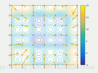
Particle swarm optimization (PSO) simulates birds in a flock of birds by designing a massless particle. The particle has only two attributes: speed and position. Speed represents the speed of movement and position represents the direction of movement. Each particle searches for the optimal solution separately in the search space, records it as the current individual extreme value, shares the individual extreme value with other particles in the whole particle swarm, and finds the optimal individual extreme value as the current global optimal solution of the whole particle swarm, All particles in the particle swarm adjust their speed and position according to the current individual extreme value found by themselves and the current global optimal solution shared by the whole particle swarm. The following dynamic diagram vividly shows the process of PSO algorithm:

2 update rules
PSO is initialized as a group of random particles (random solutions). Then the optimal solution is found by iteration. In each iteration, the particles update themselves by tracking two "extreme values" (pbest, gbest). After finding these two optimal values, the particle updates its speed and position through the following formula.

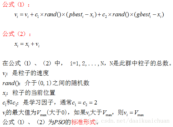
The first part of formula (1) is called [memory item], which represents the influence of the last speed and direction; The second part of formula (1) is called [self cognition item], which is a vector from the current point to the best point of the particle itself, indicating that the action of the particle comes from its own experience; The third part of formula (1) is called [group cognition item], which is a vector from the current point to the best point of the population, reflecting the cooperation and knowledge sharing among particles. Particles determine their next movement through their own experience and the best experience of their companions. Based on the above two formulas, the standard form of PSO is formed.

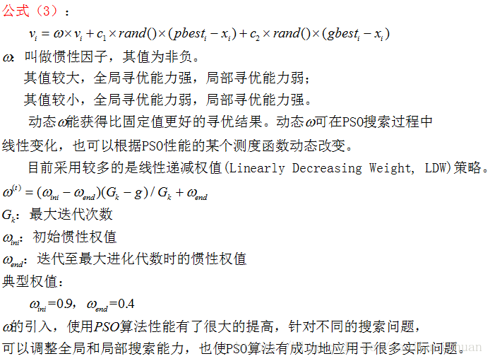
Equations (2) and (3) are considered as standard PSO algorithms.
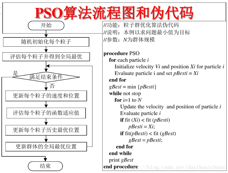
3 PSO algorithm flow and pseudo code

2, Source code

%% Clear environment variables
function chapter_PSO
close all;
clear;
clc;
format compact;
%% Data extraction



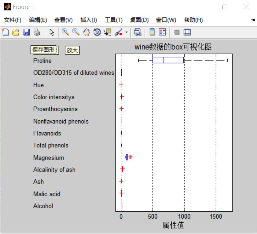
% Draw the fractal dimension visualization diagram of test data
figure
subplot(3,5,1);
hold on
for run = 1:178
    plot(run,wine_labels(run),'*');
end
xlabel('sample','FontSize',10);
ylabel('Category label','FontSize',10);
title('class','FontSize',10);
for run = 2:14
    subplot(3,5,run);
    hold on;
    str = ['attrib ',num2str(run-1)];
    for i = 1:178
        plot(i,wine(i,run-1),'*');
    end
    xlabel('sample','FontSize',10);
    ylabel('Attribute value','FontSize',10);
    title(str,'FontSize',10);
end

% Select training set and test set

% 1 of the first category-30,Class II 60-95,Class III 131-153 As a training set
train_wine = [wine(1:30,:);wine(60:95,:);wine(131:153,:)];
% The labels of the corresponding training sets should also be separated
train_wine_labels = [wine_labels(1:30);wine_labels(60:95);wine_labels(131:153)];
% 31 of the first category-59,Category II 96-130,Class III 154-178 As a test set
test_wine = [wine(31:59,:);wine(96:130,:);wine(154:178,:)];
% The label of the corresponding test set should also be separated
test_wine_labels = [wine_labels(31:59);wine_labels(96:130);wine_labels(154:178)];

%% Data preprocessing
% Data preprocessing,Normalize the training set and test set to[0,1]section

[mtrain,ntrain] = size(train_wine);
[mtest,ntest] = size(test_wine);

dataset = [train_wine;test_wine];
% mapminmax by MATLAB Self contained normalization function
[dataset_scale,ps] = mapminmax(dataset',0,1);
dataset_scale = dataset_scale';

train_wine = dataset_scale(1:mtrain,:);
test_wine = dataset_scale( (mtrain+1):(mtrain+mtest),: );
%% Choose the best SVM parameter c&g

[bestacc,bestc,bestg] = psoSVMcgForClass(train_wine_labels,train_wine);

% Print selection results
disp('Print selection results');
str = sprintf( 'Best Cross Validation Accuracy = %g%% Best c = %g Best g = %g',bestacc,bestc,bestg);
disp(str);

%% Using the best parameters SVM Network training
cmd = ['-c ',num2str(bestc),' -g ',num2str(bestg)];
model = svmtrain(train_wine_labels,train_wine,cmd);

%% SVM Network prediction
[predict_label,accuracy] = svmpredict(test_wine_labels,test_wine,model);

% Print test set classification accuracy
total = length(test_wine_labels);
right = sum(predict_label == test_wine_labels);
disp('Print test set classification accuracy');
str = sprintf( 'Accuracy = %g%% (%d/%d)',accuracy(1),right,total);
disp(str);

%% Result analysis

% Actual classification and predicted classification diagram of test set
% It can be seen from the figure that only three test samples are misclassified
figure;
hold on;
plot(test_wine_labels,'o');
plot(predict_label,'r*');
xlabel('Test set samples','FontSize',12);
ylabel('Category label','FontSize',12);
legend('Actual test set classification','Prediction test set classification');
title('Actual classification and predicted classification diagram of test set','FontSize',12);
grid on;
snapnow;

%% Subfunction psoSVMcgForClass.m
function [bestCVaccuarcy,bestc,bestg,pso_option] = psoSVMcgForClass(train_label,train,pso_option)
% psoSVMcgForClass


% Parameter initialization
if nargin == 2
    pso_option = struct('c1',1.5,'c2',1.7,'maxgen',200,'sizepop',20, ...
        'k',0.6,'wV',1,'wP',1,'v',5, ...
        'popcmax',10^2,'popcmin',10^(-1),'popgmax',10^3,'popgmin',10^(-2));
end
% c1:The initial value is 1.5,pso Parameter local search capability
% c2:The initial value is 1.7,pso Parameter global search capability
% maxgen:Initially 200,Maximum evolutionary quantity
% sizepop:Initial 20,Maximum population
% k:Initial 0.6(k belongs to [0.1,1.0]),Rate and x Relationship between(V = kX)
% wV:The initial value is 1(wV best belongs to [0.8,1.2]),Elastic coefficient in front of velocity in rate update formula
% wP:The initial value is 1,Elastic coefficient in front of velocity in population renewal formula
% v:The initial is 3,SVM Cross Validation parameter
% popcmax:Initially 100,SVM parameter c Maximum value of change in.
% popcmin:Initial 0.1,SVM parameter c Minimum value of change.
% popgmax:Initially 1000,SVM parameter g Maximum value of change.
% popgmin:Initial 0.01,SVM parameter c Minimum value of change.

Vcmax = pso_option.k*pso_option.popcmax;
Vcmin = -Vcmax ;
Vgmax = pso_option.k*pso_option.popgmax;
Vgmin = -Vgmax ;

eps = 10^(-3);

% Generate initial particles and velocities
for i=1:pso_option.sizepop
    
    % Randomly generated population and speed
    pop(i,1) = (pso_option.popcmax-pso_option.popcmin)*rand+pso_option.popcmin;
    pop(i,2) = (pso_option.popgmax-pso_option.popgmin)*rand+pso_option.popgmin;
    V(i,1)=Vcmax*rands(1,1);
    V(i,2)=Vgmax*rands(1,1);
    
    % Calculate initial fitness
    cmd = ['-v ',num2str(pso_option.v),' -c ',num2str( pop(i,1) ),' -g ',num2str( pop(i,2) )];
    fitness(i) = svmtrain(train_label, train, cmd);
    fitness(i) = -fitness(i);
end

% Find extreme value and extreme point
[global_fitness bestindex]=min(fitness); % Global extremum
local_fitness=fitness;   % Individual extremum initialization

global_x=pop(bestindex,:);   % Global extreme point
local_x=pop;    % Individual extreme point initialization

% Average fitness of each generation population
avgfitness_gen = zeros(1,pso_option.maxgen);

% Iterative optimization
for i=1:pso_option.maxgen
    
    for j=1:pso_option.sizepop
        
        %Speed update
        V(j,:) = pso_option.wV*V(j,:) + pso_option.c1*rand*(local_x(j,:) - pop(j,:)) + pso_option.c2*rand*(global_x - pop(j,:));
        if V(j,1) > Vcmax
            V(j,1) = Vcmax;
        end
        if V(j,1) < Vcmin
            V(j,1) = Vcmin;
        end
        if V(j,2) > Vgmax
            V(j,2) = Vgmax;
        end
        if V(j,2) < Vgmin
            V(j,2) = Vgmin;
        end
        
        %Population regeneration
        pop(j,:)=pop(j,:) + pso_option.wP*V(j,:);
        if pop(j,1) > pso_option.popcmax
            pop(j,1) = pso_option.popcmax;
        end
        if pop(j,1) < pso_option.popcmin
            pop(j,1) = pso_option.popcmin;
        end
        if pop(j,2) > pso_option.popgmax
            pop(j,2) = pso_option.popgmax;
        end
        if pop(j,2) < pso_option.popgmin
            pop(j,2) = pso_option.popgmin;
        end
        
        % Adaptive particle mutation
        if rand>0.5
            k=ceil(2*rand);
            if k == 1
                pop(j,k) = (20-1)*rand+1;
            end
            if k == 2
                pop(j,k) = (pso_option.popgmax-pso_option.popgmin)*rand + pso_option.popgmin;
            end
        end
        
        %Fitness value
        cmd = ['-v ',num2str(pso_option.v),' -c ',num2str( pop(j,1) ),' -g ',num2str( pop(j,2) )];
        fitness(j) = svmtrain(train_label, train, cmd);
        fitness(j) = -fitness(j);
        
        cmd_temp = ['-c ',num2str( pop(j,1) ),' -g ',num2str( pop(j,2) )];
        model = svmtrain(train_label, train, cmd_temp);
        
        if fitness(j) >= -65
            continue;
        end

3, Operation results

4, Remarks

Version: 2014a