catalogue
Find the linear regression function by gradient descent:
Several important concepts (about data processing)
linear regression
Linear regression is a statistical analysis method that uses regression analysis in mathematical statistics to determine the interdependent quantitative relationship between two or more variables. It is widely used.
Regression analysis includes only one independent variable and one dependent variable, and the relationship between them can be approximately expressed by a straight line. This regression analysis is called univariate linear regression analysis. If the regression analysis includes two or more independent variables, and there is a linear relationship between dependent variables and independent variables, it is called multiple linear regression analysis.
Univariate linear regression
From the above definition, we can know that regression analysis only includes an independent variable and a dependent variable, and the relationship between them can be approximately expressed by a straight line. This regression is called univariate linear regression analysis. Univariate linear regression is a kind of regression, and the evaluated independent variable X and dependent variable Y are linear. When there is only one independent variable, it is called univariate linear regression.
We need to know what is linear?, Generally speaking, the image we get is a straight line, and the highest order term of the independent variable is 1,
Fitting is to construct an algorithm so that the algorithm can conform to the real data.
From the perspective of machine fitting, linear regression is to construct a linear function to make the consistency between the function and the target value the best. From the perspective of space, it is necessary to make the straight line (face) of the function as close to all data points in space as possible (the sum of the distance parallel to the y axis from the point to the straight line is the shortest).
Linear regression model:

For example, if we have some data of house area and corresponding price, we can fit a straight line to make it conform to the relationship between house area and price as much as possible (that is, the sample points fall near the straight line we fit as much as possible)
So how should we fit this line? We first need to know the loss function.
loss function
Loss function is also called objective function or cost function. In short, it is a function of error. The loss function is used to measure the difference between the predicted value and the real value of the model. The goal of machine learning is to establish a loss function to minimize the value of the function.
In other words, the loss function is a function of model parameters, and the possible value combination of independent variables is usually infinite. Our goal is to find the most appropriate combination of independent variables among many possible combinations to minimize the value of the loss function.
The loss function is used to evaluate the difference between the predicted value and the real value of the model. The smaller the loss function, the better the performance of the model. The loss functions used in different models are generally different
Generally speaking, the real value of the data is used to subtract the predicted value obtained by the functional model, and the error of a sample is calculated. It is used to estimate the inconsistency between the predicted value f(x) of your model and the real value Y.
The formula is LOSS = real value - predicted value
For univariate linear regression. We usually use the mean square loss function:
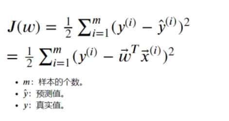
If we have a loss function, how can we find its minimum value? Here 1 we will use the gradient descent method.
gradient descent
gradient descent is widely used in machine learning. Whether in linear regression or Logistic regression, its main purpose is to find the minimum value of the objective function through iteration or converge to the minimum value.
Deflection:
In a univariate function, the derivative is the rate of change of the function. For the "rate of change" of binary function, the situation is much more complicated because there is one more independent variable.
In the xOy plane, when the moving point changes in different directions from P(x0,y0), the change speed of function f(x,y) is generally different. Therefore, it is necessary to study the change rate of f(x,y) in different directions at point (x0,y0).
Here, we only study the change rate of f(x,y) when the function f(x,y) changes along two special directions parallel to the x-axis and parallel to the y-axis.
The symbol of partial derivative is: ∂. The partial derivative reflects the rate of change of the function along the positive direction of each coordinate axis. The maximum direction of the gradient is the direction of the directional derivative, that is, the direction with the fastest numerical change.
Gradient descent;
We can use downhill as an example: (here we quote the example given by others)
Suppose such a scenario: a person is trapped on a mountain and needs to come down from the mountain (find the lowest point of the mountain, that is, the valley). But at this time, the dense fog on the mountain is very large, resulting in low visibility; Therefore, the path down the mountain cannot be determined. We must use the information around us to find the way down the mountain step by step. At this time, you can use the gradient descent algorithm to help yourself down the mountain. How to do it? First, take his current position as the benchmark, find the steepest place in this position, then take a step in the downward direction, and then continue to take his current position as the benchmark, find the steepest place, and then walk until he finally reaches the lowest place;
In short: Generally speaking, it is to use the information of the current location to iterate step by step to find the location of the minimum value.
According to our knowledge of high numbers, the direction along the derivative is the maximum direction of numerical change. Therefore, derivation is essential. Just like going down the mountain, when we have the direction of going down the mountain, we should consider the steps we have taken down the mountain. The step size is also an important parameter in the gradient descent. When we have the direction of going down the mountain and the step size of going down the mountain, we can go step by step to the bottom of the mountain, that is, the parameters of the minimum value point in the function we want to require.
The following is a schematic diagram of one dimension and multi dimension:

General steps of gradient descent:

Let's look at two specific examples: (using gradient descent to find the lowest point of the function)
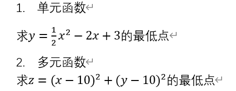
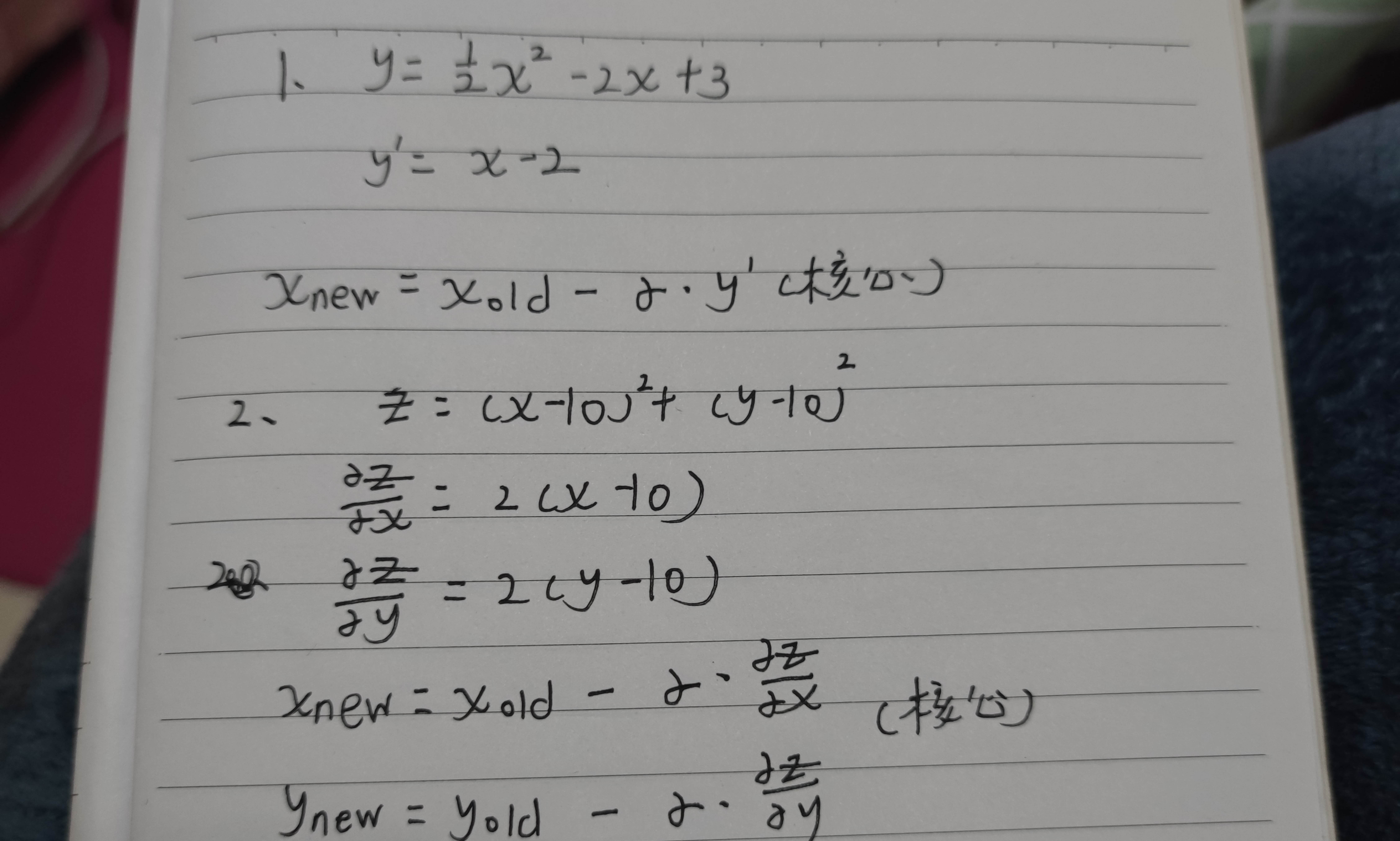
Manual derivation:
Code example:
Unitary situation:
import numpy as np
import matplotlib.pyplot as plt
plot_x=np.linspace(-1,6,141)   #The number of generated 141 equidistant between - 1 and 6
 # At the same time, according to plot_x to generate plot_y
plot_y=0.5*plot_x*plot_x-2*plot_x+3
plt.plot(plot_x,plot_y)
plt.show()
###Define a function dJ for finding the derivative of a quadratic function
def dJ(x):
    return x-2

###Define a function J for finding the value of the function
def J(x):
    try:
        return 0.5*x*x-2*x+3
    except:
        return float('inf')
x=0.0							#Pick a starting point at random
eta=0.1		#Learning rate
i=0
epsilon=1e-8				    #A condition used to determine whether the minimum point of a quadratic function is reached
history_x=[x]                   #Used to record the X coordinate of the point passed by the gradient descent method
while True:
    i=i+1
    d=0.5*x*x-2*x+3
    gradient=dJ(x)				#Gradient (derivative)
    last_x=x
    x=x-eta*gradient
    print("The first%d Second iteration function value%f x coordinate%f Rate of change%f"%(i,J(last_x),x,abs(J(last_x)-J(x))))
    history_x.append(x)
    if (abs(J(last_x)-J(x)) <epsilon):		#Used to judge whether it approaches the lowest point
        break
print(history_x)	        #Print the value of x when the lowest point is reached
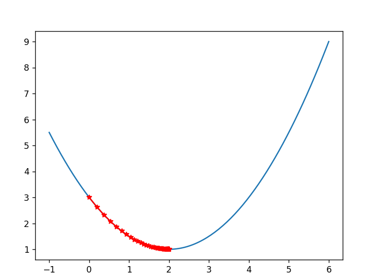
plt.plot(plot_x,plot_y)
plt.plot(np.array(history_x),J(np.array(history_x)),color='r',marker='*')   #Draw the track of x
plt.show()
Image replacement:
Binary situation:
import numpy as np
import matplotlib.pyplot as plt
from mpl_toolkits.mplot3d import Axes3D
#Define the derivative of x
def dJx(x):
    return 2*x-20
#Define the derivative of y
def dJy(y):
    return 2*y-20
#Define evaluation function
def z(x,y):
    return (x-10)**2+(y-10)**2
x=100.0
eta=0.1
i=0
k=0
y=100.0
epsilon=1e-8
historz_x=[x]
historz_y=[y]
m=z(x,y)
z1=[]
z1.append(m)
while True:
    i=i+1
    #dz=(x-10)**2+(y-10)**2
    gradientx=dJx(x)		#x gradient (derivative)
    gradienty=dJy(y)
    last_x=x
    last_y=y
    x=x-eta*gradientx
    y=y-eta*gradienty
    print("The first%d Second iteration function value%f x coordinate%f y coordinate%f  Rate of change%f " %(i,z(last_x,last_y),x,y,abs(z(last_x,last_y)-z(x,y))))
    historz_x.append(x)
    historz_y.append(y)
    m=z(x,y)
    z1.append(m)
    if (abs(z(last_x,last_y)-z(x,y)) <epsilon):		#Used to judge whether it approaches the lowest point
        break
print(historz_x)#Print the value of x when the lowest point is reached
print(historz_y)#Print the value of y when the lowest point is reached
print(z1)

fig = plt.figure()
ax = fig.add_subplot(projection='3d')
#ax = Axes3D(plt.figure())

# Generate the coordinate set (- 2,2) interval of X and y with an interval of 0.1
x = np.arange(-100, 100, 0.1)
y = np.arange(-100, 100.,0.1)

# Generate grid
X, Y = np.meshgrid(x, y)

# Z-axis function
Z =(X-10)**2+(Y -10)**2
# Define x,y axis names
plt.xlabel("x")
plt.ylabel("y")
# Set spacing and color
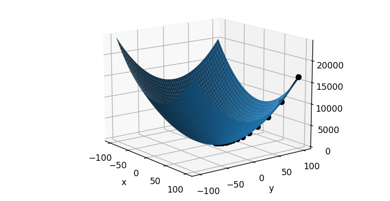
ax.plot_surface(X, Y, Z)
ax.plot(historz_x,historz_y,z1,'ko', lw=2, ls='-')
# Exhibition
plt.show()
Image changes:
Find the linear regression function by gradient descent:

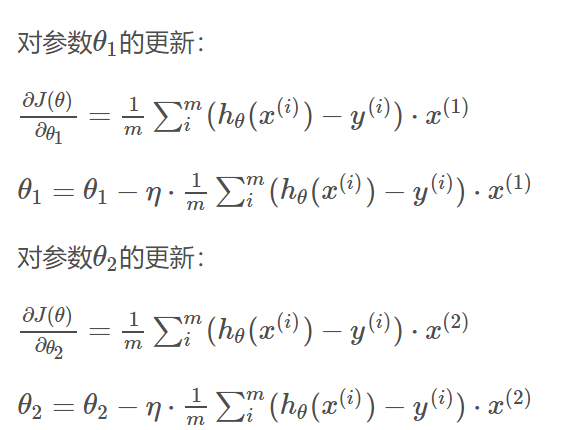
Main steps of parameter update:
1. Randomly initialize a set of parameters θ
2. Set the objective function J( θ) J( θ) For each parameter θ Find the partial derivative (which can also be understood as the fastest direction down the mountain at each current position)
3. Subtract the derivative of the old value from the old value and multiply it by the step to get the new value.
θnew=θold-a *f'(θold)
a is learning efficiency (also can be understood as the pace of going down the mountain)
b is the change of X in each iteration ; b= θ old- θ new.
4. The number of iterations is generally controlled by two parameters
The initial number of cycles {or when b, that is, the change is less than a specific value. Note: a can be set by itself. It is not easy to be too large or too small. Too large is easy to cause inaccuracy, and too small is easy to cause too many iterations.
Let's look at a specific example: (use gradient descent to find the minimum point parameter of loss function)
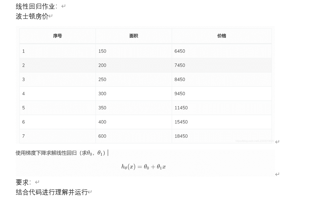
Let's continue to look at an example of linear regression (a job):
Code example
import math
m=7 #Dataset size
alpha=0.000001#Learning rate
area=[150,200,250,300,350,400,600];#data set
price=[6450,7450,8450,9450,11450,15450,18450];
def gradientx(Theta0,Theta1):#Partial derivative of Theta0
    ans=0
    for i in range(0,7):
        ans=ans+Theta0+Theta1*area[i]-price[i]
    ans=ans/m
    return ans
def gradienty(Theta0,Theta1):#Partial derivative of Theta1 0
    ans=0
    for i in range(0,7):
        ans=ans+(Theta0+Theta1*area[i]-price[i])*area[i]
    ans=ans/m
    return ans
def loss(Theta0,Theta1):  #loss function
    ans=0
    for i in range(0,7):
        ans=ans+pow((Theta0+Theta1*area[i]-price[i]),2)
    ans=ans/(2*m)
    return ans
nowTheta0=1700  #Initial value set
nowTheta1=60
print('Set parameters at')
print(nowTheta0,nowTheta1)
#while math.fabs(nowTheta1-Theta1) >0.0000001 :#gradient descent
for i in range(500000):
    nowa=nowTheta0
    nowTheta0 = nowTheta0-alpha*gradientx(nowTheta0,nowTheta1)
    nowTheta1 = nowTheta1-alpha*gradienty(nowa, nowTheta1)
    if loss(nowTheta0,nowTheta1)<100.0:
        break
print('Fitting parameters')
print(nowTheta0,nowTheta1 )
import numpy as np
from matplotlib import pyplot
area=[150,200,250,300,350,400,600]#data set
price=[6450,7450,8450,9450,11450,15450,18450]
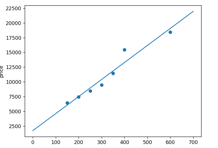
pyplot.scatter(area,price)
x=np.arange(0,700,0.1) #Value of random production X
y=nowTheta1*x+nowTheta0
pyplot.plot(x,y)
pyplot.xlabel('area')
pyplot.ylabel('price')
pyplot.show()
Fitting results:
Several important concepts (about data processing)
1. Normalization:

2. Standardization:

3. Regularization:
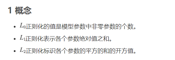
The details are here( (1 message) understanding of regularization_ Blog that has never gone far - CSDN blog_ Regularization)
Several common libraries:
The usage of the following libraries will not be described in detail here.
import pandas as pd
import numpy as np (used to process array matrix)
Introduction to common numpy usage( (1 message) use of numpy Library of python learning notes -- sup er detailed_ Dream following blog - CSDN blog_ How to import numpy and name it np)
import matplotlib. Pyplot as plot (used for drawing data visualization)
Introduction to the usage of common matplotlib Libraries( (1 message) Python--Matplotlib (basic usage)_ Hard boat man - CSDN blog_ matplotlib)