
Artificial intelligence learning is inseparable from the verification of practice. It is recommended that you can learn more in Flyai AI competition service platform Take part in more training and competitions to improve your ability. FlyAI is a one-stop service platform that provides AI developers with data competition and supports GPU offline training. Provide free open source algorithm samples of the project every week to support algorithm capability realization and fast iterative algorithm model.
Introduction to pytorch
Pytorch is one of the two most popular machine learning frameworks in the world at present, which is in parallel with tens of low. It provides many convenient functions, such as how to adjust the parameters according to the automatic differential calculation of loss, a series of mathematical function encapsulation, a series of ready-made models and the framework of combining the models for training. The predecessor of pytorch is torch, which is based on lua, while pytorch is based on python. Although it is based on python, the bottom layer is completely written in c + +. It supports automatic parallelization calculation and GPU acceleration, so its performance is very good.
Some of the traditional machine learning will be like the example in the previous section, all handwriting, or use numpy class library to reduce part of the workload, while others will use various classical algorithms encapsulated by scikit learn (based on numpy) class library. Unlike tensorflow and traditional machine learning, pytorch focuses on building a neural network similar to human brain, so it can realize very complex judgments that traditional machine learning cannot do, such as judging the type of object in the picture, automatic driving, etc. However, there is still a lot of controversy about whether the working mode of the neural network they build is really similar to that of the human brain. At present, some people have begun to build a GNN (Graph Neural Network) network that is closer to the human brain in principle, but it has not yet been practical. Therefore, our series will focus on the network models that have been practical and widely used in various industries.
Is it better to learn pytorch or tensorflow?
A common question for beginners is, is it better to learn pytorch or tensorflow? According to the current statistics, companies use tensorflow more, while researchers use pytorch more. The growth rate of pytorch is very fast, which has a trend to surpass tensorflow. My opinion is that it doesn't matter which one to learn. If you are familiar with pytorch, learning tensorflow will take a day or two, and vice versa. In addition, the projects of pytorch and tensorflow can be transplanted to each other. Just choose one that feels easy to learn. Because I think pytorch is better to learn (the encapsulation is very intuitive, and using Dynamic Graph makes debugging very easy), this series will be based on pytorch.
Dynamic Graph and Static Graph
Machine learning framework can be divided into Dynamic Graph and Static Graph according to whether the operation process needs to be fixed in advance. Dynamic Graph does not need to fix the operation process in advance, but Static Graph does. For example, for the same formula wx + b = y, the Dynamic Graph framework can write wx and + b separately and calculate step by step. During the calculation process, you can output the results on the way with instructions such as , print , or send the results on the way to other places for recording; The Static Graph framework must pre-set the whole calculation process. You can only pass in w, x, b to the calculator, and then let the calculator output y. The results of Midway calculation can only be viewed by a special debugger.
Generally speaking, the performance of Static Graph is better than that of Dynamic Graph. Tensorflow (the old version) uses Static Graph and pytorch uses Dynamic Graph, but the actual performance difference between them is very small, because most of the resources consumed are matrix operations, and the use of batch training can greatly reduce their gap. Incidentally, Tensorflow 1.7 supports Dynamic Graph and is enabled by default in 2.0, but most people still use Static Graph when using tensorflow.
# According to the impression of Dynamic Graph, custom code can be inserted at every step of operation
def forward(w, x, b):
    wx = w * x
    print(wx)
    y = wx + b
    print(y)
    return y
forward(w, x, b)

# According to the impression of Static Graph, the whole calculation process needs to be compiled in advance
forward = compile("wx+b")
forward(w, x, b)
Install pytorch
Assuming that you have installed python3, you can install pytorch by executing the following command:
pip3 install pytorch
Then, you can reference the python class library by using import torch in the Python code.
Basic operation of pytorch
Next, let's get familiar with the most basic operations in pytorch. Pytorch will use {torch Tensor , type is used to uniformly represent values, vectors (one-dimensional array) or matrices (multi-dimensional array). This type will also be used for model parameters. (tensorflow can be divided into several types according to the purpose, which pytorch is more concise)
torch. Tensor , type can use , torch The tensor # function is built. The following are some simple examples (running in python REPL):
# Reference pytorch
>>> import torch

# Create an integer tensor
>>> torch.tensor(1)
tensor(1)

# Create a decimal tensor
>>> torch.tensor(1.0)
tensor(1.)

# The value in the single valued tensor can be retrieved with the item function
>>> torch.tensor(1.0).item()
1.0

# Create a vector tensor using a one-dimensional array
>>> torch.tensor([1.0, 2.0, 3.0])
tensor([1., 2., 3.])

# Create a matrix tensor using a two-dimensional array
>>> torch.tensor([[1.0, 2.0, 3.0], [-1.0, -2.0, -3.0]])
tensor([[ 1.,  2.,  3.],
        [-1., -2., -3.]])
The numeric type of the tensor object can be seen from its {dtype} members:
>>> torch.tensor(1).dtype
torch.int64
>>> torch.tensor(1.0).dtype
torch.float32
>>> torch.tensor([1.0, 2.0, 3.0]).dtype
torch.float32
>>> torch.tensor([[1.0, 2.0, 3.0], [-1.0, -2.0, -3.0]]).dtype
torch.float32
pytorch supports integer type {torch uint8, torch.int8, torch.int16, torch.int32, torch.int64, floating-point number type, {torch float16, torch.float32, torch.float64, and the boolean type {torch bool. The number after the type represents its number of bits (bit number), while the # u # before # uint8 # represents that it is an unsigned number. In fact, most of the scenes only use {torch Float32, although the accuracy is not {torch Float64 # is high, but it takes up less memory and has fast operation speed. Note that only one type of values can be saved in a tensor object, and cannot be mixed.
When creating a tensor object, you can force the type to be specified through the {dtype} parameter:
>>> torch.tensor(1, dtype=torch.int32)
tensor(1, dtype=torch.int32)
>>> torch.tensor([1.1, 2.9, 3.5], dtype=torch.int32)
tensor([1, 2, 3], dtype=torch.int32)

>>> torch.tensor(1, dtype=torch.int64)
tensor(1)

>>> torch.tensor(1, dtype=torch.float32)
tensor(1.)

>>> torch.tensor(1, dtype=torch.float64)
tensor(1., dtype=torch.float64)
>>> torch.tensor([1, 2, 3], dtype=torch.float64)
tensor([1., 2., 3.], dtype=torch.float64)

>>> torch.tensor([1, 2, 0], dtype=torch.bool)
tensor([ True,  True, False])
The shape of the tensor object can be seen from its # shape # members:
# shape of integer tensor is null
>>> torch.tensor(1).shape
torch.Size([])
>>> torch.tensor(1.0).shape
torch.Size([])

# The shape of the array tensor has only one value, which represents the length of the array
>>> torch.tensor([1.0]).shape
torch.Size([1])
>>> torch.tensor([1.0, 2.0, 3.0]).shape
torch.Size([3])

# The shape of the matrix tensor depends on its dimensions. Each value represents the size of each dimension. This example represents that the matrix has two rows and three columns
>>> torch.tensor([[1.0, 2.0, 3.0], [-1.0, -2.0, -3.0]]).shape
torch.Size([2, 3])
Tensor object and numerical value. Operations can be performed between tensor object and tensor object:
>>> torch.tensor(1.0) * 2
tensor(2.)
>>> torch.tensor(1.0) * torch.tensor(2.0)
tensor(2.)
>>> torch.tensor(3.0) * torch.tensor(2.0)
tensor(6.)
Vectors and matrices can also be operated in batches (parallelization operation will be performed internally):
# Operation between vector and value
>>> torch.tensor([1.0, 2.0, 3.0])
tensor([1., 2., 3.])
>>> torch.tensor([1.0, 2.0, 3.0]) * 3
tensor([3., 6., 9.])
>>> torch.tensor([1.0, 2.0, 3.0]) * 3 - 1
tensor([2., 5., 8.])

# Operation between matrix and single valued tensor object
>>> torch.tensor([[1.0, 2.0, 3.0], [-1.0, -2.0, -3.0]])
tensor([[ 1.,  2.,  3.],
        [-1., -2., -3.]])
>>> torch.tensor([[1.0, 2.0, 3.0], [-1.0, -2.0, -3.0]]) / torch.tensor(2)
tensor([[ 0.5000,  1.0000,  1.5000],
        [-0.5000, -1.0000, -1.5000]])

# The operation between a matrix and a vector of the same length as the last dimension of the matrix
>>> torch.tensor([[1.0, 2.0, 3.0], [-1.0, -2.0, -3.0]]) * torch.tensor([1.0, 1.5, 2.0])
tensor([[ 1.,  3.,  6.],
        [-1., -3., -6.]])
The operation between tensor objects will generally generate a new tensor object. If you want to avoid generating new objects (improve performance), you can use_ At the end of the function, they will modify the original object:
# Generate a new object, the original object remains unchanged, and add and + have the same meaning
>>> a = torch.tensor([1,2,3])
>>> b = torch.tensor([7,8,9])
>>> a.add(b)
tensor([ 8, 10, 12])
>>> a
tensor([1, 2, 3])

# Perform operations on the original object to avoid generating new objects
>>> a.add_(b)
tensor([ 8, 10, 12])
>>> a
tensor([ 8, 10, 12])
pytorch also provides a series of convenient functions to calculate the maximum value, minimum value, average value, standard deviation, etc
>>> torch.tensor([1.0, 2.0, 3.0])
tensor([1., 2., 3.])
>>> torch.tensor([1.0, 2.0, 3.0]).min()
tensor(1.)
>>> torch.tensor([1.0, 2.0, 3.0]).max()
tensor(3.)
>>> torch.tensor([1.0, 2.0, 3.0]).mean()
tensor(2.)
>>> torch.tensor([1.0, 2.0, 3.0]).std()
tensor(1.)
pytorch also supports comparing tensor objects to generate tensors of boolean type:
# Comparison between tensor object and numerical value
>>> torch.tensor([1.0, 2.0, 3.0]) > 1.0
tensor([False,  True,  True])
>>> torch.tensor([1.0, 2.0, 3.0]) <= 2.0
tensor([ True,  True, False])

# Comparison between tensor object and tensor object
>>> torch.tensor([1.0, 2.0, 3.0]) > torch.tensor([1.1, 1.9, 3.0])
tensor([False,  True, False])
>>> torch.tensor([1.0, 2.0, 3.0]) <= torch.tensor([1.1, 1.9, 3.0])
tensor([ True, False,  True])
pytorch also supports the generation of tensor objects with specified shapes:
# Generate a matrix tensor with 2 rows and 3 columns, and all values are 0
>>> torch.zeros(2, 3)
tensor([[0., 0., 0.],
        [0., 0., 0.]])

# Generate a matrix tensor with 3 rows and 2 columns, all of which are 1
torch.ones(3, 2)
>>> torch.ones(3, 2)
tensor([[1., 1.],
        [1., 1.],
        [1., 1.]])

# Generate a matrix tensor with 3 rows and 2 columns, all of which are 100
>>> torch.full((3, 2), 100)
tensor([[100., 100.],
        [100., 100.],
        [100., 100.]])

# Generate a matrix tensor with 3 rows and 3 columns, and the value is a random floating-point number in the range [0,1]
>>> torch.rand(3, 3)
tensor([[0.4012, 0.2412, 0.1532],
        [0.1178, 0.2319, 0.4056],
        [0.7879, 0.8318, 0.7452]])

# Generate a matrix tensor with 3 rows and 3 columns, and the value is a random integer in the range [1, 10]
>>> (torch.rand(3, 3) * 10 + 1).long()
tensor([[ 8,  1,  5],
        [ 8,  6,  5],
        [ 1,  6, 10]])

# The effect is the same as the above writing
>>> torch.randint(1, 11, (3, 3))
tensor([[7, 1, 3],
        [7, 9, 8],
        [4, 7, 3]])
The operations mentioned here are only a common part. If you want to know more about the operations supported by the tensor object, you can refer to the following documents:
pytorch saves the data structure used by tensor
In order to reduce memory usage and improve access speed, pytorch will use a continuous storage space (whether in system memory or GPU memory) to save tensor s, whether they are numeric, vector or matrix.
We can use , storage , to view the storage space used by the tensor object:
# The storage space length of the value is 1
>>> torch.tensor(1).storage()
 1
[torch.LongStorage of size 1]

# The length of the storage space of the vector is equal to the length of the vector
>>> torch.tensor([1, 2, 3], dtype=torch.float32).storage()
 1.0
 2.0
 3.0
[torch.FloatStorage of size 3]

# The storage space length of the matrix is equal to the result of multiplying all dimensions. Here are 2 rows and 3 columns, with a total of 6 elements
>>> torch.tensor([[1, 2, 3], [-1, -2, -3]], dtype=torch.float64).storage()
 1.0
 2.0
 3.0
 -1.0
 -2.0
 -3.0
[torch.DoubleStorage of size 6]
pytorch will use string to determine the dimension of a tensor object:
# The storage space has 6 elements
>>> torch.tensor([[1, 2, 3], [-1, -2, -3]]).storage()
 1
 2
 3
 -1
 -2
 -3
[torch.LongStorage of size 6]

# The first dimension is 2 and the second dimension is 3 (2 rows and 3 columns)
>>> torch.tensor([[1, 2, 3], [-1, -2, -3]]).shape
torch.Size([2, 3])

# The meaning of stripe is to represent the distance between elements in each dimension
# The first dimension will be divided into 3 elements (6 elements can be divided into 2 groups), and the second dimension will be divided into 1 element (3 elements)
>>> torch.tensor([[1, 2, 3], [-1, -2, -3]])
tensor([[ 1,  2,  3],
        [-1, -2, -3]])
>>> torch.tensor([[1, 2, 3], [-1, -2, -3]]).stride()
(3, 1)
A powerful feature of pytorch is that you can modify the dimension of the tensor object through the # view # function (the # stripe is changed internally), but you do not need to create a new storage space and copy elements:
# Create a matrix with 2 rows and 3 columns
>>> a = torch.tensor([[1, 2, 3], [-1, -2, -3]])
>>> a
tensor([[ 1,  2,  3],
        [-1, -2, -3]])
>>> a.shape
torch.Size([2, 3])
>>> a.stride()
(3, 1)

# Change the dimension to 3 rows and 2 columns
>>> b = a.view(3, 2)
>>> b
tensor([[ 1,  2],
        [ 3, -1],
        [-2, -3]])
>>> b.shape
torch.Size([3, 2])
>>> b.stride()
(2, 1)

# Convert to vector
>>> c = b.view(6)
>>> c
tensor([ 1,  2,  3, -1, -2, -3])
>>> c.shape
torch.Size([6])
>>> c.stride()
(1,)

# Their storage space is the same
>>> a.storage()
 1
 2
 3
 -1
 -2
 -3
[torch.LongStorage of size 6]
>>> b.storage()
 1
 2
 3
 -1
 -2
 -3
[torch.LongStorage of size 6]
>>> c.storage()
 1
 2
 3
 -1
 -2
 -3
[torch.LongStorage of size 6]
Another meaning of using , stripe , to determine the dimension is that it can support sharing the same space to realize the transpose operation:
# Create a matrix with 2 rows and 3 columns
>>> a = torch.tensor([[1, 2, 3], [-1, -2, -3]])
>>> a
tensor([[ 1,  2,  3],
        [-1, -2, -3]])
>>> a.shape
torch.Size([2, 3])
>>> a.stride()
(3, 1)

# Swap dimensions using transpose (row to column)
>>> b = a.transpose(0, 1)
>>> b
tensor([[ 1, -1],
        [ 2, -2],
        [ 3, -3]])
>>> b.shape
torch.Size([3, 2])
>>> b.stride()
(1, 3)

# Their storage space is the same
>>> a.storage()
 1
 2
 3
 -1
 -2
 -3
[torch.LongStorage of size 6]
>>> b.storage()
 1
 2
 3
 -1
 -2
 -3
[torch.LongStorage of size 6]
The internal transpose operation is to exchange the corresponding values of the specified dimension in the "string". You can think about how the objects will be divided in the transposed matrix according to the previous description.
Now think again, if the transposed matrix is designed as a vector with the , view , function, why will it change? Will it become [1, - 1, 2, - 2, 3, - 3]?
In fact, such an operation will lead to an error 😱:
>>> b
tensor([[ 1, -1],
        [ 2, -2],
        [ 3, -3]])
>>> b.view(6)
Traceback (most recent call last):
  File "<stdin>", line 1, in <module>
RuntimeError: view size is not compatible with input tensor's size and stride (at least one dimension spans across two contiguous subspaces). Use .reshape(...) instead.
This is because the natural order of matrix elements after transpose is inconsistent with the order in the storage space. We can use {is_ Use the continuous} function to detect:
>>> a.is_contiguous()
True
>>> b.is_contiguous()
False
The way to solve this problem is to copy another copy of the storage space with the # continuous # function to make the order consistent, and then use the # view # function to change the dimension; Or use the more convenient , reshape , function. Reshape , function will detect whether the storage space needs to be copied when changing the dimension. If necessary, copy. If not, just modify the internal , stripe like , view ,.
>>> b.contiguous().view(6)
tensor([ 1, -1,  2, -2,  3, -3])
>>> b.reshape(6)
tensor([ 1, -1,  2, -2,  3, -3])
pytorch also supports intercepting part of the storage space as a new tensor object, based on the internal storage_ The offset and size attributes also do not need to be copied:
# Examples of intercepting vectors
>>> a = torch.tensor([1, 2, 3, -1, -2, -3])
>>> b = a[1:3]
>>> b
tensor([2, 3])
>>> b.storage_offset()
1
>>> b.size()
torch.Size([2])
>>> b.storage()
 1
 2
 3
 -1
 -2
 -3
[torch.LongStorage of size 6]

# Example of intercepting matrix
>>> a.view(3, 2)
tensor([[ 1,  2],
        [ 3, -1],
        [-2, -3]])
>>> c = a.view(3, 2)[1:] # The first dimension (line) intercepts 1~ the end, and the second dimension does not intercept
>>> c
tensor([[ 3, -1],
        [-2, -3]])
>>> c.storage_offset()
2
>>> c.size()
torch.Size([2, 2])
>>> c.stride()
(2, 1)
>>> c.storage()
 1
 2
 3
 -1
 -2
 -3
[torch.LongStorage of size 6]

# The example of intercepted transposed matrix is more complex
>>> a.view(3, 2).transpose(0, 1)
tensor([[ 1,  3, -2],
        [ 2, -1, -3]])
>>> c = a.view(3, 2).transpose(0, 1)[:,1:] # The first dimension (row) is not intercepted, and the second dimension (column) is intercepted 1~ at the end
>>> c
tensor([[ 3, -2],
        [-1, -3]])
>>> c.storage_offset()
2
>>> c.size()
torch.Size([2, 2])
>>> c.stride()
(1, 2)
>>> c.storage()
 1
 2
 3
 -1
 -2
 -3
[torch.LongStorage of size 6]
Well, after reading this section, you should have a basic understanding of how pytorch stores tensor objects. In order to make it easy to understand, this section only uses two-dimensional matrices as examples at most. You can try whether more dimensional matrices can operate in the same way.
Introduction to matrix multiplication
Next, let's look at matrix multiplication, which is the most frequent operation in machine learning. What we learned in high school and remember should be reviewed,
The following is a simple example. A matrix with two rows and three columns can be multiplied by a matrix with three rows and four columns to obtain a matrix with two rows and four columns:
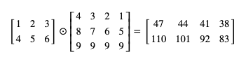
Matrix multiplication will take the total value of each row of the first matrix multiplied by each column of the second matrix as the result, which can be understood by referring to the following figure:
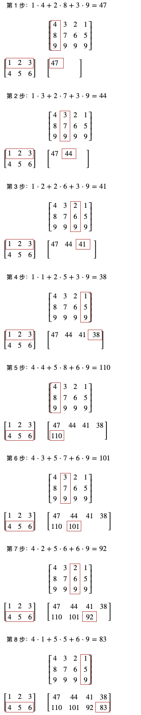
According to this rule, if a matrix with n rows and m columns is multiplied by a matrix with M rows and p columns, a matrix with n rows and p columns will be obtained (the number of columns of the first matrix and the number of rows of the second matrix must be the same).
What's the point of matrix multiplication? The significance of matrix multiplication in machine learning is that the calculation of multiple inputs and outputs or intermediate values can be combined into one operation (the formula can also be greatly simplified mathematically). The framework can calculate in parallel internally, because the high-end GPU has thousands of cores. Distributing the calculation into thousands of cores can greatly improve the operation speed. In the following example, you can also see how to use matrix multiplication to realize batch training.
Matrix multiplication calculation using pytorch
In pytorch, matrix multiplication can call the {mm} function:
>>> a = torch.tensor([[1,2,3],[4,5,6]])
>>> b = torch.tensor([[4,3,2,1],[8,7,6,5],[9,9,9,9]])
>>> a.mm(b)
tensor([[ 47,  44,  41,  38],
        [110, 101,  92,  83]])

# If the size does not match, an error occurs
>>> a = torch.tensor([[1,2,3],[4,5,6]])
>>> b = torch.tensor([[4,3,2,1],[8,7,6,5]])
>>> a.mm(b)
Traceback (most recent call last):
  File "<stdin>", line 1, in <module>
RuntimeError: size mismatch, m1: [2 x 3], m2: [2 x 4] at ../aten/src/TH/generic/THTensorMath.cpp:197

# The mm function can also be replaced by the @ operator, and the result is the same
>>> a = torch.tensor([[1,2,3],[4,5,6]])
>>> b = torch.tensor([[4,3,2,1],[8,7,6,5],[9,9,9,9]])
>>> a @ b
tensor([[ 47,  44,  41,  38],
        [110, 101,  92,  83]])
For matrix multiplication of more dimensions, pytorch provides the {mathul} function:
# Multiply the matrix of n x m by the matrix of q x m x p to get the matrix of q x n x p
>>> a = torch.ones(2,3)
>>> b = torch.ones(5,3,4)
>>> a.matmul(b)
tensor([[[3., 3., 3., 3.],
         [3., 3., 3., 3.]],

        [[3., 3., 3., 3.],
         [3., 3., 3., 3.]],

        [[3., 3., 3., 3.],
         [3., 3., 3., 3.]],

        [[3., 3., 3., 3.],
         [3., 3., 3., 3.]],

        [[3., 3., 3., 3.],
         [3., 3., 3., 3.]]])
>>> a.matmul(b).shape
torch.Size([5, 2, 4])
Automatic differentiation function of pytorch (autograd)
pytorch supports automatic differential derivation function value (i.e. the gradient of each parameter). Using this function, we no longer need to calculate the derivation function value of each parameter through mathematical formula, which makes the threshold of machine learning much lower 😄😄, The following is an example of this function:
# Define parameters
# Set the requirements when creating the tensor object_ Grad is True to turn on the automatic differentiation function
>>> w = torch.tensor(1.0, requires_grad=True)
>>> b = torch.tensor(0.0, requires_grad=True)

# Define tensor s for input and output
>>> x = torch.tensor(2)
>>> y = torch.tensor(5)

# Calculate prediction output
>>> p = x * w + b
>>> p
tensor(2., grad_fn=<AddBackward0>)

# Calculate loss
# Note that the automatic differential function of pytorch requires that the loss cannot be negative, because pytorch only considers reducing the loss rather than making the loss close to 0
# abs is used here to make the loss absolute
>>> l = (p - y).abs()
>>> l
tensor(3., grad_fn=<AbsBackward>)

# Deriving function value from loss automatic differentiation
>>> l.backward()

# Check the leading function value corresponding to each parameter
# Note that pytorch assumes that the loss can be reduced only by subtracting the value of grad from the parameter, so this is a negative number (the parameter will become larger)
>>> w.grad
tensor(-2.)
>>> b.grad
tensor(-1.)

# Define the learning ratio, that is, the ratio of adjusting the parameters according to the derivative value each time
>>> learning_rate = 0.01

# Torch is needed to adjust parameters no_ Grad temporarily disables the automatic differentiation function
>>> with torch.no_grad():
...     w -= w.grad * learning_rate
...     b -= b.grad * learning_rate
...

# We can see that weight and bias increased by 0.02 and 0.01 respectively
>>> w
tensor(1.0200, requires_grad=True)
>>> b
tensor(0.0100, requires_grad=True)

# Finally, we need to clear the grad value of the parameter, which will not be cleared automatically (because some models need to superimpose the derivative value)
# You can try adjusting backward again, and you will find that grad superimposes the two values
>>> w.grad.zero_()
>>> b.grad.zero_()
Let's try the method mentioned in the previous section to make the loss equal to the square of the difference value:
# Define parameters
>>> w = torch.tensor(1.0, requires_grad=True)
>>> b = torch.tensor(0.0, requires_grad=True)

# Define tensor s for input and output
>>> x = torch.tensor(2)
>>> y = torch.tensor(5)

# Calculate prediction output
>>> p = x * w + b
>>> p
tensor(2., grad_fn=<AddBackward0>)

# Calculate the difference value
>>> d = p - y
>>> d
tensor(-3., grad_fn=<SubBackward0>)

# Calculate the loss (the square of the difference value must be 0 or positive)
>>> l = d ** 2
>>> l
tensor(9., grad_fn=<PowBackward0>)

# Deriving function value from loss automatic differentiation
>>> l.backward()

# Check the corresponding derivative value of each parameter, which is the same as the value obtained by mathematical formula in the previous article
# Derivative value of w = 2 * d * x = 2 * -3 * 2 = -12
# Derivative value of b = 2 * d = 2 * -3 = -6
>>> w.grad
tensor(-12.)
>>> b.grad
tensor(-6.)

# Then adjust the parameters as in the previous example
Greasy and harmful 😼, No matter how complex the model is, it can automatically help us calculate the derivative function value by calling backward. From now on, we can throw away the mathematics textbook (this is a joke. Some problems still need to be understood in mathematics, but in most cases, people with only basic mathematics knowledge can afford to play).
Loss function of pytorch
pytorch provides the encapsulation of several common loss calculators. What we first saw is also called L1 loss, which represents the average of the absolute value of the difference between all predicted outputs and correct outputs (there will be multiple outputs in some scenarios). The following is an example of using L1 loss:
# Define parameters
>>> w = torch.tensor(1.0, requires_grad=True)
>>> b = torch.tensor(0.0, requires_grad=True)

# Define tensor s for input and output
# Note that the loss calculator provided by pytorch requires both the predicted output and the correct output to be floating-point numbers, so floating-point numbers are also required when defining input and output
>>> x = torch.tensor(2.0)
>>> y = torch.tensor(5.0)

# Create loss calculator
>>> loss_function = torch.nn.L1Loss()

# Calculate prediction output
>>> p = x * w + b
>>> p
tensor(2., grad_fn=<AddBackward0>)

# Calculate loss
# Equivalent to (P - y) abs(). mean()
>>> l = loss_function(p, y)
>>> l
tensor(3., grad_fn=<L1LossBackward>)
Calculating the square of the difference value as the loss is called MSE loss (Mean Squared Error), which is also called L2 loss in some places. The following is an example of using MSE loss:
# Define parameters
>>> w = torch.tensor(1.0, requires_grad=True)
>>> b = torch.tensor(0.0, requires_grad=True)

# Define tensor s for input and output
>>> x = torch.tensor(2.0)
>>> y = torch.tensor(5.0)

# Create loss calculator
>>> loss_function = torch.nn.MSELoss()

# Calculate prediction output
>>> p = x * w + b
>>> p
tensor(2., grad_fn=<AddBackward0>)

# Calculate loss
# Equivalent to ((P - y) * * 2) mean()
>>> l = loss_function(p, y)
>>> l
tensor(9., grad_fn=<MseLossBackward>)
Convenient bell 🙂 In addition, if you want to see more loss calculators, you can refer to the following address:
pytorch's parameter adjuster package (optimizer)
pytorch also provides the encapsulation of the regulator that adjusts the parameters according to the derivation value. The method we saw in these two articles (randomly initializing the parameter value and then adjusting the parameters according to the derivation value * learning ratio to reduce the loss) is also known as the stochastic gradient descent method. The following is an example of using the encapsulated regulator:
# Define parameters
>>> w = torch.tensor(1.0, requires_grad=True)
>>> b = torch.tensor(0.0, requires_grad=True)

# Define tensor s for input and output
>>> x = torch.tensor(2.0)
>>> y = torch.tensor(5.0)

# Create loss calculator
>>> loss_function = torch.nn.MSELoss()

# Create parameter adjuster
# You need to pass in the parameter list and specify the learning ratio. The learning ratio here is 0.01
>>> optimizer = torch.optim.SGD([w, b], lr=0.01)

# Calculate prediction output
>>> p = x * w + b
>>> p
tensor(2., grad_fn=<AddBackward0>)

# Calculate loss
>>> l = loss_function(p, y)
>>> l
tensor(9., grad_fn=<MseLossBackward>)

# Deriving function value from loss automatic differentiation
>>> l.backward()

# Confirm the derivative value of the parameter
>>> w.grad
tensor(-12.)
>>> b.grad
tensor(-6.)

# Use the parameter adjuster to adjust the parameters
# Equivalent to:
# with torch.no_grad():
#     w -= w.grad * learning_rate
#     b -= b.grad * learning_rate
optimizer.step()

# Clear leading function value
# Equivalent to:
# w.grad.zero_()
# b.grad.zero_()
optimizer.zero_grad()

# Confirm the adjusted parameters
>>> w
tensor(1.1200, requires_grad=True)
>>> b
tensor(0.0600, requires_grad=True)
>>> w.grad
tensor(0.)
>>> b.grad
tensor(0.)
The learning ratio of SGD parameter regulator is fixed. If we want to automatically adjust the learning ratio during the learning process, we can use other parameter regulators, such as Adam regulator. In addition, you can also turn on the momentum option to improve the learning speed. After this option is turned on, you can refer to the direction (plus or minus) of the previous adjustment when adjusting the parameters. If it is the same, you can adjust more, while if it is different, you can adjust less.
If you are interested in the implementation of Adam adjuster and impulse, you can refer to the following articles (you need some mathematical knowledge):
If you want to view other parameter adjusters provided by pytorch, you can visit the following address:
Using pytorch to implement the example of the previous article
Well, after learning this, we should have a certain understanding of the basic operation of pytorch. Now let's try to implement the last example of the last article.
The final example code of the previous article is as follows:
# Define parameters
weight = 1
bias = 0

# Define learning ratio
learning_rate = 0.01

# Prepare training set, verification set and test set
traning_set = [(2, 5), (5, 11), (6, 13), (7, 15), (8, 17)]
validating_set = [(12, 25), (1, 3)]
testing_set = [(9, 19), (13, 27)]

# Record the historical values of weight and bias
weight_history = [weight]
bias_history = [bias]

for epoch in range(1, 10000):
    print(f"epoch: {epoch}")

    # Train and modify the parameters according to the training set
    for x, y in traning_set:
        # Calculate predicted value
        predicted = x * weight + bias
        # Calculate loss
        diff = predicted - y
        loss = diff ** 2
        # Print debug information
        print(f"traning x: {x}, y: {y}, predicted: {predicted}, loss: {loss}, weight: {weight}, bias: {bias}")
        # Calculate the derivative value
        derivative_weight = 2 * diff * x
        derivative_bias = 2 * diff
        # Modify weight and bias to reduce loss
        # When diff is positive, it means predicted output > correct output, which will reduce weight and bias
        # When diff is negative, it means that the predicted output < the correct output, which will increase weight and bias
        weight -= derivative_weight * learning_rate
        bias -= derivative_bias * learning_rate
        # Record the historical values of weight and bias
        weight_history.append(weight)
        bias_history.append(bias)

    # Check validation set
    validating_accuracy = 0
    for x, y in validating_set:
        predicted = x * weight + bias
        validating_accuracy += 1 - abs(y - predicted) / y
        print(f"validating x: {x}, y: {y}, predicted: {predicted}")
    validating_accuracy /= len(validating_set)

    # If the correct rate of the verification set is greater than 99%, stop the training
    print(f"validating accuracy: {validating_accuracy}")
    if validating_accuracy > 0.99:
        break

# Check test set
testing_accuracy = 0
for x, y in testing_set:
    predicted = x * weight + bias
    testing_accuracy += 1 - abs(y - predicted) / y
    print(f"testing x: {x}, y: {y}, predicted: {predicted}")
testing_accuracy /= len(testing_set)
print(f"testing accuracy: {testing_accuracy}")

# Show the changes of weight and bias
from matplotlib import pyplot
pyplot.plot(weight_history, label="weight")
pyplot.plot(bias_history, label="bias")
pyplot.legend()
pyplot.show()
After using pytorch, the code is as follows:
# Reference pytorch
import torch

# Define parameters
weight = torch.tensor(1.0, requires_grad=True)
bias = torch.tensor(0.0, requires_grad=True)

# Create loss calculator
loss_function = torch.nn.MSELoss()

# Create parameter adjuster
optimizer = torch.optim.SGD([weight, bias], lr=0.01)

# Prepare training set, verification set and test set
traning_set = [
    (torch.tensor(2.0), torch.tensor(5.0)),
    (torch.tensor(5.0), torch.tensor(11.0)),
    (torch.tensor(6.0), torch.tensor(13.0)),
    (torch.tensor(7.0), torch.tensor(15.0)),
    (torch.tensor(8.0), torch.tensor(17.0))
]
validating_set = [
    (torch.tensor(12.0), torch.tensor(25.0)),
    (torch.tensor(1.0), torch.tensor(3.0))
]
testing_set = [
    (torch.tensor(9.0), torch.tensor(19.0)),
    (torch.tensor(13.0), torch.tensor(27.0))
]

# Record the historical values of weight and bias
weight_history = [weight.item()]
bias_history = [bias.item()]

for epoch in range(1, 10000):
    print(f"epoch: {epoch}")

    # Train and modify the parameters according to the training set
    for x, y in traning_set:
        # Calculate predicted value
        predicted = x * weight + bias
        # Calculate loss
        loss = loss_function(predicted, y)
        # Print debug information
        print(f"traning x: {x}, y: {y}, predicted: {predicted}, loss: {loss}, weight: {weight}, bias: {bias}")
        # Deriving function value from loss automatic differentiation
        loss.backward()
        # Use the parameter adjuster to adjust the parameters
        optimizer.step()
        # Clear leading function value
        optimizer.zero_grad()
        # Record the historical values of weight and bias
        weight_history.append(weight.item())
        bias_history.append(bias.item())

    # Check validation set
    validating_accuracy = 0
    for x, y in validating_set:
        predicted = x * weight.item() + bias.item()
        validating_accuracy += 1 - abs(y - predicted) / y
        print(f"validating x: {x}, y: {y}, predicted: {predicted}")
    validating_accuracy /= len(validating_set)

    # If the correct rate of the verification set is greater than 99%, stop the training
    print(f"validating accuracy: {validating_accuracy}")
    if validating_accuracy > 0.99:
        break

# Check test set
testing_accuracy = 0
for x, y in testing_set:
    predicted = x * weight.item() + bias.item()
    testing_accuracy += 1 - abs(y - predicted) / y
    print(f"testing x: {x}, y: {y}, predicted: {predicted}")
testing_accuracy /= len(testing_set)
print(f"testing accuracy: {testing_accuracy}")

# Show the changes of weight and bias
from matplotlib import pyplot
pyplot.plot(weight_history, label="weight")
pyplot.plot(bias_history, label="bias")
pyplot.legend()
pyplot.show()
The output is as follows:
epoch: 1
traning x: 2.0, y: 5.0, predicted: 2.0, loss: 9.0, weight: 1.0, bias: 0.0
traning x: 5.0, y: 11.0, predicted: 5.659999847412109, loss: 28.515602111816406, weight: 1.1200000047683716, bias: 0.05999999865889549
traning x: 6.0, y: 13.0, predicted: 10.090799331665039, loss: 8.463448524475098, weight: 1.6540000438690186, bias: 0.16679999232292175
traning x: 7.0, y: 15.0, predicted: 14.246713638305664, loss: 0.5674403309822083, weight: 2.0031042098999023, bias: 0.22498400509357452
traning x: 8.0, y: 17.0, predicted: 17.108564376831055, loss: 0.011786224320530891, weight: 2.1085643768310547, bias: 0.24004973471164703
validating x: 12.0, y: 25.0, predicted: 25.33220863342285
validating x: 1.0, y: 3.0, predicted: 2.3290724754333496
validating accuracy: 0.8815345764160156
epoch: 2
traning x: 2.0, y: 5.0, predicted: 4.420266628265381, loss: 0.3360907733440399, weight: 2.0911941528320312, bias: 0.2378784418106079
traning x: 5.0, y: 11.0, predicted: 10.821391105651855, loss: 0.03190113604068756, weight: 2.1143834590911865, bias: 0.24947310984134674
traning x: 6.0, y: 13.0, predicted: 13.04651165008545, loss: 0.002163333585485816, weight: 2.132244348526001, bias: 0.25304529070854187
traning x: 7.0, y: 15.0, predicted: 15.138755798339844, loss: 0.019253171980381012, weight: 2.1266629695892334, bias: 0.25211507081985474
traning x: 8.0, y: 17.0, predicted: 17.107236862182617, loss: 0.011499744839966297, weight: 2.1072371006011963, bias: 0.24933995306491852
validating x: 12.0, y: 25.0, predicted: 25.32814598083496
validating x: 1.0, y: 3.0, predicted: 2.3372745513916016
validating accuracy: 0.8829828500747681
epoch: 3
traning x: 2.0, y: 5.0, predicted: 4.427353858947754, loss: 0.32792359590530396, weight: 2.0900793075561523, bias: 0.24719521403312683
traning x: 5.0, y: 11.0, predicted: 10.82357406616211, loss: 0.0311261098831892, weight: 2.112985134124756, bias: 0.2586481273174286
traning x: 6.0, y: 13.0, predicted: 13.045942306518555, loss: 0.002110695466399193, weight: 2.1306276321411133, bias: 0.26217663288116455
traning x: 7.0, y: 15.0, predicted: 15.137059211730957, loss: 0.018785227090120316, weight: 2.1251144409179688, bias: 0.2612577974796295
traning x: 8.0, y: 17.0, predicted: 17.105924606323242, loss: 0.011220022104680538, weight: 2.105926036834717, bias: 0.2585166096687317
validating x: 12.0, y: 25.0, predicted: 25.324134826660156
validating x: 1.0, y: 3.0, predicted: 2.3453762531280518
validating accuracy: 0.8844133615493774

Omit output in transit

epoch: 202
traning x: 2.0, y: 5.0, predicted: 4.950470924377441, loss: 0.0024531292729079723, weight: 2.0077908039093018, bias: 0.9348894953727722
traning x: 5.0, y: 11.0, predicted: 10.984740257263184, loss: 0.00023285974748432636, weight: 2.0097720623016357, bias: 0.9358800649642944
traning x: 6.0, y: 13.0, predicted: 13.003972053527832, loss: 1.5777208318468183e-05, weight: 2.0112979412078857, bias: 0.9361852407455444
traning x: 7.0, y: 15.0, predicted: 15.011855125427246, loss: 0.00014054399798624218, weight: 2.0108213424682617, bias: 0.9361057877540588
traning x: 8.0, y: 17.0, predicted: 17.00916290283203, loss: 8.39587883092463e-05, weight: 2.0091617107391357, bias: 0.9358686804771423
validating x: 12.0, y: 25.0, predicted: 25.028034210205078
validating x: 1.0, y: 3.0, predicted: 2.9433810710906982
validating accuracy: 0.9900028705596924
testing x: 9.0, y: 19.0, predicted: 19.004947662353516
testing x: 13.0, y: 27.0, predicted: 27.035730361938477
testing accuracy: 0.9992080926895142
The same training succeeded 😼. You may find that the output value is somewhat different from that in the previous article. This is because python uses 32-bit floating point number (float32) by default, while python uses 64 bit floating point number (float64). If you change the part of parameter definition to this:
# Define parameters
weight = torch.tensor(1.0, dtype=torch.float64, requires_grad=True)
bias = torch.tensor(0.0, dtype=torch.float64, requires_grad=True)
Then change the part of calculating the loss to this way, and you can get the same output as the previous article:
# Calculate loss
loss = loss_function(predicted, y.double())
Batch training using matrix multiplication
Although the previous example uses pytorch to realize the training, it is still a value calculation. We can use matrix multiplication to realize batch training and calculate multiple values at a time. The following modified code:
# Reference pytorch
import torch

# Define parameters
weight = torch.tensor([[1.0]], requires_grad=True) # 1 row 1 column
bias = torch.tensor(0.0, requires_grad=True)

# Create loss calculator
loss_function = torch.nn.MSELoss()

# Create parameter adjuster
optimizer = torch.optim.SGD([weight, bias], lr=0.01)

# Prepare training set, verification set and test set
traning_set_x = torch.tensor([[2.0], [5.0], [6.0], [7.0], [8.0]]) # Five rows and one column represent five groups with one input in each group
traning_set_y = torch.tensor([[5.0], [11.0], [13.0], [15.0], [17.0]]) # Five rows and one column represent five groups with one output in each group
validating_set_x = torch.tensor([[12.0], [1.0]]) # Two rows and one column represent two groups with one input in each group
validating_set_y = torch.tensor([[25.0], [3.0]]) # Two rows and one column represent two groups with one output in each group
testing_set_x = torch.tensor([[9.0], [13.0]]) # Two rows and one column represent two groups with one input in each group
testing_set_y = torch.tensor([[19.0], [27.0]]) # Two rows and one column represent two groups with one output in each group

# Record the historical values of weight and bias
weight_history = [weight[0][0].item()]
bias_history = [bias.item()]

for epoch in range(1, 10000):
    print(f"epoch: {epoch}")

    # Train and modify the parameters according to the training set

    # Calculate predicted value
    # Multiply the matrix with 5 rows and 1 column by the matrix with 1 row and 1 column to obtain the matrix with 5 rows and 1 column
    predicted = traning_set_x.mm(weight) + bias
    # Calculate loss
    loss = loss_function(predicted, traning_set_y)
    # Print debug information
    print(f"traning x: {traning_set_x}, y: {traning_set_y}, predicted: {predicted}, loss: {loss}, weight: {weight}, bias: {bias}")
    # Deriving function value from loss automatic differentiation
    loss.backward()
    # Use the parameter adjuster to adjust the parameters
    optimizer.step()
    # Clear leading function value
    optimizer.zero_grad()
    # Record the historical values of weight and bias
    weight_history.append(weight[0][0].item())
    bias_history.append(bias.item())

    # Check validation set
    with torch.no_grad(): # Disable automatic differentiation function
        predicted = validating_set_x.mm(weight) + bias
        validating_accuracy = 1 - ((validating_set_y - predicted).abs() / validating_set_y).mean()
    print(f"validating x: {validating_set_x}, y: {validating_set_y}, predicted: {predicted}")

    # If the correct rate of the verification set is greater than 99%, stop the training
    print(f"validating accuracy: {validating_accuracy}")
    if validating_accuracy > 0.99:
        break

# Check test set
with torch.no_grad(): # Disable automatic differentiation function
    predicted = testing_set_x.mm(weight) + bias
    testing_accuracy = 1 - ((testing_set_y - predicted).abs() / testing_set_y).mean()
print(f"testing x: {testing_set_x}, y: {testing_set_y}, predicted: {predicted}")
print(f"testing accuracy: {testing_accuracy}")

# Show the changes of weight and bias
from matplotlib import pyplot
pyplot.plot(weight_history, label="weight")
pyplot.plot(bias_history, label="bias")
pyplot.legend()
pyplot.show()
The output is as follows:
epoch: 1
traning x: tensor([[2.],
        [5.],
        [6.],
        [7.],
        [8.]]), y: tensor([[ 5.],
        [11.],
        [13.],
        [15.],
        [17.]]), predicted: tensor([[2.],
        [5.],
        [6.],
        [7.],
        [8.]], grad_fn=<AddBackward0>), loss: 47.79999923706055, weight: tensor([[1.]], requires_grad=True), bias: 0.0
validating x: tensor([[12.],
        [ 1.]]), y: tensor([[25.],
        [ 3.]]), predicted: tensor([[22.0200],
        [ 1.9560]])
validating accuracy: 0.7663999795913696
epoch: 2
traning x: tensor([[2.],
        [5.],
        [6.],
        [7.],
        [8.]]), y: tensor([[ 5.],
        [11.],
        [13.],
        [15.],
        [17.]]), predicted: tensor([[ 3.7800],
        [ 9.2520],
        [11.0760],
        [12.9000],
        [14.7240]], grad_fn=<AddBackward0>), loss: 3.567171573638916, weight: tensor([[1.8240]], requires_grad=True), bias: 0.13199999928474426
validating x: tensor([[12.],
        [ 1.]]), y: tensor([[25.],
        [ 3.]]), predicted: tensor([[24.7274],
        [ 2.2156]])
validating accuracy: 0.8638148307800293

Omit output in transit

epoch: 1103
traning x: tensor([[2.],
        [5.],
        [6.],
        [7.],
        [8.]]), y: tensor([[ 5.],
        [11.],
        [13.],
        [15.],
        [17.]]), predicted: tensor([[ 4.9567],
        [10.9867],
        [12.9966],
        [15.0066],
        [17.0166]], grad_fn=<AddBackward0>), loss: 0.0004764374461956322, weight: tensor([[2.0100]], requires_grad=True), bias: 0.936755359172821
validating x: tensor([[12.],
        [ 1.]]), y: tensor([[25.],
        [ 3.]]), predicted: tensor([[25.0564],
        [ 2.9469]])
validating accuracy: 0.99001544713974
testing x: tensor([[ 9.],
        [13.]]), y: tensor([[19.],
        [27.]]), predicted: tensor([[19.0265],
        [27.0664]])
testing accuracy: 0.998073160648346
Huh? How did it take 1103 times to train successfully this time? This is because the adjustment direction of weight and bias is always the same, so only one batch of training will be slower. In the following article, we will use more parameters (neurons) to train, and they can have different adjustment directions, so the problem in this example will not appear. Of course, sometimes in business, the training is slow or cannot converge because the parameter adjustment directions are all the same. At this time, we can solve the problem by changing the model or dividing multiple batches.
Examples of dividing training set, verification set and test set
The above example defines the training set, verification set and test set one by one. Do you think it's very troublesome? We can divide them more conveniently through the tensor operation provided by pytorch:
# Raw data set
>>> dataset = [(1, 3), (2, 5), (5, 11), (6, 13), (7, 15), (8, 17), (9, 19), (12, 25), (13, 27)]

# Convert the original data set to tensor, and specify the value type as floating point number
>>> dataset_tensor = torch.tensor(dataset, dtype=torch.float32)
>>> dataset_tensor
tensor([[ 1.,  3.],
        [ 2.,  5.],
        [ 5., 11.],
        [ 6., 13.],
        [ 7., 15.],
        [ 8., 17.],
        [ 9., 19.],
        [12., 25.],
        [13., 27.]])

# Assign an initial value to the random number generator so that each run can generate the same random number
# This is to make the training process repeatable, or you can choose not to do so
>>> torch.random.manual_seed(0)
<torch._C.Generator object at 0x10cc03070>

# Generate random index value, which is used to disrupt the data order and prevent uneven distribution
>>> dataset_tensor.shape
torch.Size([9, 2])
>>> random_indices = torch.randperm(dataset_tensor.shape[0])
>>> random_indices
tensor([8, 0, 2, 3, 7, 1, 4, 5, 6])

# Calculate the index value list of training set, verification set and test set
# 60% of the data is divided into training set, 20% into verification set and 20% into test set
>>> traning_indices = random_indices[:int(len(random_indices)*0.6)]
>>> traning_indices
tensor([8, 0, 2, 3, 7])
>>> validating_indices = random_indices[int(len(random_indices)*0.6):int(len(random_indices)*0.8):]
>>> validating_indices
tensor([1, 4])
>>> testing_indices = random_indices[int(len(random_indices)*0.8):]
>>> testing_indices
tensor([5, 6])

# Divide training set, verification set and test set
>>> traning_set_x = dataset_tensor[traning_indices][:,:1] # The first dimension does not intercept, and the second dimension intercepts elements with an index value less than 1
>>> traning_set_y = dataset_tensor[traning_indices][:,1:] # The first dimension does not intercept, and the second dimension intercepts elements whose index value is greater than or equal to 1
>>> traning_set_x
tensor([[13.],
        [ 1.],
        [ 5.],
        [ 6.],
        [12.]])
>>> traning_set_y
tensor([[27.],
        [ 3.],
        [11.],
        [13.],
        [25.]])
>>> validating_set_x = dataset_tensor[validating_indices][:,:1]
>>> validating_set_y = dataset_tensor[validating_indices][:,1:]
>>> validating_set_x
tensor([[2.],
        [7.]])
>>> validating_set_y
tensor([[ 5.],
        [15.]])
>>> testing_set_x = dataset_tensor[testing_indices][:,:1]
>>> testing_set_y = dataset_tensor[testing_indices][:,1:]
>>> testing_set_x
tensor([[8.],
        [9.]])
>>> testing_set_y
tensor([[17.],
        [19.]])
The code is as follows:
# Raw data set
dataset = [(1, 3), (2, 5), (5, 11), (6, 13), (7, 15), (8, 17), (9, 19), (12, 25), (13, 27)]

# Convert original dataset to tensor
dataset_tensor = torch.tensor(dataset, dtype=torch.float32)

# Assign an initial value to the random number generator so that each run can generate the same random number
torch.random.manual_seed(0)

# Segmentation training set, verification set and test set
random_indices = torch.randperm(dataset_tensor.shape[0])
traning_indices = random_indices[:int(len(random_indices)*0.6)]
validating_indices = random_indices[int(len(random_indices)*0.6):int(len(random_indices)*0.8):]
testing_indices = random_indices[int(len(random_indices)*0.8):]
traning_set_x = dataset_tensor[traning_indices][:,:1]
traning_set_y = dataset_tensor[traning_indices][:,1:]
validating_set_x = dataset_tensor[validating_indices][:,:1]
validating_set_y = dataset_tensor[validating_indices][:,1:]
testing_set_x = dataset_tensor[testing_indices][:,:1]
testing_set_y = dataset_tensor[testing_indices][:,1:]
Note that changing the data distribution can affect the training speed. You can try how many times the above code can be trained successfully (up to 99% accuracy). However, the more and more uniform the data, the less the influence of the distribution on the training speed.
Define model class (torch.nn.Module)
What should we do if we want to provide our own model to others, or use the model written by others? pytorch provides the basic class for encapsulating the model nn. Module, the model in the above example can be rewritten as follows:
# Reference pytorch and match lotlib used to display charts
import torch
from matplotlib import pyplot

# Define model
# The model needs to define a forward function to receive input and return predicted output
# add_history and show_history is a custom function, which is only used to help us understand the principle of machine learning. In fact, it is not necessary to do so
class MyModle(torch.nn.Module):
    def __init__(self):
        # Initialize base class
        super().__init__()
        # Define parameters
        # Torch. Is required nn. Parameter packing, requires_grad doesn't need to be set (it will be set for us)
        self.weight = torch.nn.Parameter(torch.tensor([[1.0]]))
        self.bias = torch.nn.Parameter(torch.tensor(0.0))
        # Record the historical values of weight and bias
        self.weight_history = [self.weight[0][0].item()]
        self.bias_history = [self.bias.item()]

    def forward(self, x):
        # Calculate predicted value
        predicted = x.mm(self.weight) + self.bias
        return predicted

    def add_history(self):
        # Record the historical values of weight and bias
        self.weight_history.append(self.weight[0][0].item())
        self.bias_history.append(self.bias.item())

    def show_history(self):
        # Show the changes of weight and bias
        pyplot.plot(self.weight_history, label="weight")
        pyplot.plot(self.bias_history, label="bias")
        pyplot.legend()
        pyplot.show()

# Create model instance
model = MyModle()

# Create loss calculator
loss_function = torch.nn.MSELoss()

# Create parameter adjuster
# Calling the parameters function can automatically recursively obtain the parameter list in the model (note that recursive acquisition can also be supported in nested models)
optimizer = torch.optim.SGD(model.parameters(), lr=0.01)

# Raw data set
dataset = [(1, 3), (2, 5), (5, 11), (6, 13), (7, 15), (8, 17), (9, 19), (12, 25), (13, 27)]

# Convert original dataset to tensor
dataset_tensor = torch.tensor(dataset, dtype=torch.float32)

# Assign an initial value to the random number generator so that each run can generate the same random number
# This is to make the training process repeatable, or you can choose not to do so
torch.random.manual_seed(0)

# Segmentation training set, verification set and test set
random_indices = torch.randperm(dataset_tensor.shape[0])
traning_indices = random_indices[:int(len(random_indices)*0.6)]
validating_indices = random_indices[int(len(random_indices)*0.6):int(len(random_indices)*0.8):]
testing_indices = random_indices[int(len(random_indices)*0.8):]
traning_set_x = dataset_tensor[traning_indices][:,:1]
traning_set_y = dataset_tensor[traning_indices][:,1:]
validating_set_x = dataset_tensor[validating_indices][:,:1]
validating_set_y = dataset_tensor[validating_indices][:,1:]
testing_set_x = dataset_tensor[testing_indices][:,:1]
testing_set_y = dataset_tensor[testing_indices][:,1:]

# Start the training process
for epoch in range(1, 10000):
    print(f"epoch: {epoch}")

    # Train and modify the parameters according to the training set
    # Switching the model to training mode will enable automatic differentiation, batchnorm and Dropout
    model.train()

    # Calculate predicted value
    predicted = model(traning_set_x)
    # Calculate loss
    loss = loss_function(predicted, traning_set_y)
    # Print debug information
    print(f"traning x: {traning_set_x}, y: {traning_set_y}, predicted: {predicted}, loss: {loss}, weight: {model.weight}, bias: {model.bias}")
    # Deriving function value from loss automatic differentiation
    loss.backward()
    # Use the parameter adjuster to adjust the parameters
    optimizer.step()
    # Clear leading function value
    optimizer.zero_grad()
    # Record the historical values of weight and bias
    model.add_history()

    # Check validation set
    # Switching the model to validation mode will disable automatic differentiation, batchnorm and Dropout
    model.eval()
    predicted = model(validating_set_x)
    validating_accuracy = 1 - ((validating_set_y - predicted).abs() / validating_set_y).mean()
    print(f"validating x: {validating_set_x}, y: {validating_set_y}, predicted: {predicted}")

    # If the correct rate of the verification set is greater than 99%, stop the training
    print(f"validating accuracy: {validating_accuracy}")
    if validating_accuracy > 0.99:
        break

# Check test set
predicted = model(testing_set_x)
testing_accuracy = 1 - ((testing_set_y - predicted).abs() / testing_set_y).mean()
print(f"testing x: {testing_set_x}, y: {testing_set_y}, predicted: {predicted}")
print(f"testing accuracy: {testing_accuracy}")

# Show the changes of weight and bias
model.show_history()
The following points need to be paid attention to when defining and using model classes:
- Must be in constructor__ init__ Call super (). init__ () initialize the base class (this is also required for general python inheritance classes)
- The {forward} function must be defined to receive input and return predicted output
- Parameters defined in the model need to use {torch nn. Parameter packing, requires_grad # no need to set (it will be set for us)
- Call {model Parameters () can recursively obtain the parameter list (support nested models), which is required when creating parameter adjusters
- Call model. before training. Train() enables automatic differentiation and other functions
- Call model. before validating or using a trained model.eval # turn off automatic differentiation and other functions
When we continue to use pytorch for machine learning later, the structure of the code will be basically the same as the above example, except that the model is different from the inspection verification set and the test set. In addition, functions such as batch normalization and Dropout will be introduced in later articles.
This is the end of this article. I believe you have mastered the basic mode of machine learning with pytorch 😼.
Write at the end
The things introduced in this article are also very basic, but these foundations are essential for applied machine learning. The contents of these two articles are not mentioned in many machine learning tutorials. They start directly from the multi-layer linear model, so many people will complain that it is difficult to get started 😫. If you read the official book "deep learning with Python" published by pytorch, you may find that the introduction order of these two articles is very close to that of this book. Yes, I refer to this book when writing these two articles, and it is the easiest to understand them in this order.

For more articles on artificial intelligence, please visit: Flyai AI competition service platform Learning circle learning; At the same time, FlyAI welcomes the majority of Algorithm Engineers to post on the platform and get more original awards. In addition, the FlyAI competition platform provides a large number of data-based competition questions for the participation of learning parties and competition parties, free GPU trial, and more competition experience sharing.