1, Introduction

1 origin and development of ant colony algorithm (ACA)
In the process of studying the new algorithm, Marco Dorigo and others found that when ant colony is looking for food, they can exchange foraging information by secreting a biological hormone called pheromone, so they can quickly find the target. Therefore, in their doctoral thesis in 1991, they systematically proposed a new intelligent optimization algorithm "Ant system (AS) based on ant population for the first time. Later, The proposer and many researchers have made various improvements to the algorithm and applied it to a wider range of fields, such AS graph coloring problem, quadratic assignment problem, workpiece scheduling problem, vehicle routing problem, job shop scheduling problem, network routing problem, large-scale integrated circuit design and so on. In recent years, M.Dorigo and others have further developed ant algorithm into a general optimization technology "Ant Colony Optimization (ACO)", and called all algorithms in line with ACO framework "ACO algorithm".

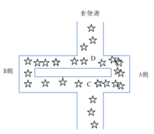
Specifically, each ant starts looking for food without telling where the food is in advance. When one finds food, it will release a volatile secretion pheromone (called pheromone, which will gradually volatilize and disappear over time. The pheromone concentration represents the distance of the path). Pheromone can be perceived by other ants and play a guiding role. Usually, when there are pheromones on multiple paths, ants will preferentially choose the path with high pheromone concentration, so that the pheromone concentration of the path with high concentration is higher, forming a positive feedback. Some ants do not always repeat the same path as other ants. They will find another way. If the other path is shorter than the original one, then gradually, more ants are attracted to this shorter path. Finally, after a period of operation, the shortest path may be repeated by most ants. Finally, the path with the highest pheromone concentration is the optimal path finally selected by ants.
Compared with other algorithms, ant colony algorithm is a relatively young algorithm, which has the characteristics of distributed computing, no central control, asynchronous and indirect communication between individuals, and is easy to be combined with other optimization algorithms. After the continuous exploration of many people with lofty ideals, a variety of improved ant colony algorithms have been developed today, but the principle of ant colony algorithm is still the backbone.

2. Solution principle of ant colony algorithm
Based on the above description of ant colony foraging behavior, the algorithm mainly simulates the foraging behavior in the following aspects:
(1) The simulated graph scene contains two pheromones, one represents home and the other represents the location of food, and both pheromones are volatilizing at a certain rate.
(2) Each ant can only perceive information in a small part of its surroundings. When ants are looking for food, if they are within the perceptual range, they can go directly. If they are not within the perceptual range, they should go to the place with more pheromones. Ants can have a small probability not to go to the place with more pheromones and find another way. This small probability event is very important, which represents an innovation in finding a way and is very important for finding a better solution.
(3) The rules for ants to return to their nest are the same as those for finding food.
(4) When moving, the ant will first follow the guidance of pheromone. If there is no guidance of pheromone, it will go inertia according to its moving direction, but there is also a certain chance to change the direction. The ant can also remember the road it has traveled and avoid going to one place again.
(5) Ants leave the most pheromones when they find food, and then the farther away from the food, the less pheromones they leave. The rules for finding the amount of pheromone left in the nest are the same as those of food. Ant colony algorithm has the following characteristics: positive feedback algorithm, concurrency algorithm, strong robustness, probabilistic global search, independent of strict mathematical properties, long search time and easy to stop.
Ant transfer probability formula:

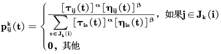
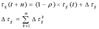
In the formula: is the probability of ant k transferring from city i to j; α，β The relative importance of pheromones and heuristic factors; Is the pheromone quantity on edge (i,j); Is heuristic factor; Select the city allowed for ant k next step. The above formula is the pheromone update formula in ant system, which is the amount of pheromone on edge (i,j); ρ Is pheromone evaporation coefficient, 0< ρ< 1; Is the pheromone quantity of the kth ant left on the edge (i,j) in this iteration; Q is a normal coefficient; Is the path length of the kth ant in this tour.
In ant system, pheromone update formula is:

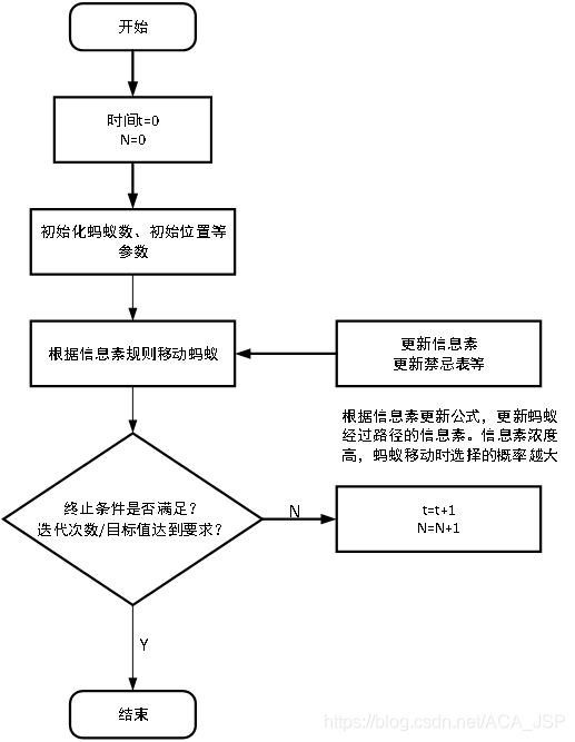
3. Solving steps of ant colony algorithm:
(1) Initialization parameters at the beginning of calculation, relevant parameters need to be initialized, such as ant colony size (number of ants) m and pheromone importance factor α, Heuristic function importance factor β, Pheromone will send Silver ρ, Total pheromone release Q, maximum number of iterations iter_max, initial value of iteration times iter=1.
(2) The solution space is constructed. Each ant is randomly placed at different starting points. For each ant K (k=1,2,3... m), the next city to be visited is calculated according to (2-1) until all ants have visited all cities.
(3) Update the information, calculate the path length Lk(k=1,2,..., m) of each ant, and record the optimal solution (shortest path) in the current number of iterations. At the same time, the pheromone concentration on each urban connection path is updated according to equations (2-2) and (2-3).
(4) Judge whether to terminate if ITER < ITER_ Max, then make iter=iter+1, clear the record table of ant passing path, and return to step 2; Otherwise, the calculation is terminated and the optimal solution is output.
(5) Judge whether to terminate if ITER < ITER_ Max, then make iter=iter+1, clear the record table of ant passing path, and return to step 2; Otherwise, the calculation is terminated and the optimal solution is output. 3. Judge whether to terminate if ITER < ITER_ Max, then make iter=iter+1, clear the record table of ant passing path, and return to step 2; Otherwise, the calculation is terminated and the optimal solution is output.

2, Source code

clc %Clear command line window
clear %Deletes all variables from the current workspace and frees them from system memory
close all %Delete all windows whose handles are not hidden
tic % Save current time
%% Ant colony algorithm CDVRP
%Input:
%City           Longitude and latitude of demand point
%Distance       Distance matrix
%Demand         Demand at each demand point
%AntNum         Population number
%Alpha          Pheromone importance factor
%Beta           Heuristic function importance factor
%Rho            Pheromone volatilization factor
%Q              Constant coefficient
%Eta            Heuristic function
%Tau            Pheromone matrix
%MaxIter        Maximum number of iterations


%Output:
%bestroute      Shortest path
%mindisever     path length 

%% Load data
load('City.mat')	      %The longitude and latitude of the demand point is used to draw the actual path XY coordinate
load('Distance.mat')	  %Distance matrix
load('Demand.mat')       %requirement
load('Travelcon.mat')	  %Travel constraint
load('Capacity.mat')     %Vehicle capacity constraint

%% Initialize problem parameters
CityNum = size(City,1)-1;    %Number of demand points

%% Initialization parameters
AntNum = 8;                            % Ant number 
Alpha = 1;                              % Pheromone importance factor
Beta = 5;                               % Heuristic function importance factor
Rho = 0.1;                              % Pheromone volatilization factor
Q = 1;                                  % Constant coefficient
Eta = 1./Distance;                      % Heuristic function
Tau = ones(CityNum+1);                  % (CityNum+1)*(CityNum+1)The pheromone matrix is initialized to 1
Population = zeros(AntNum,CityNum*2+1);  % AntNum that 's ok,(CityNum*2+1)Path record table for column
MaxIter = 100;                           % Maximum number of iterations
bestind = ones(1,CityNum*2+1);	% Best path of each generation
MinDis = zeros(MaxIter,1);              % The length of the best path of each generation

%% Iterative search for the best path
Iter = 1;                               % Initial value of iteration times
while Iter <= MaxIter %When the maximum number of iterations is not reached
	%% Ant by ant path selection
    
	for i = 1:AntNum
        TSProute=2:CityNum+1; %Generate an ascending order that does not include the first and last bits TSP Route
        VRProute=[]; %initialization VRP route
        
        while ~isempty(TSProute)%Open up new sub paths
            subpath=1; %First put the distribution center into the starting point of the sub path
            DisTraveled=0; %The distance of this sub path is initialized to zero
            delivery=0; %The vehicle deliverable quantity of this sub path is initialized to zero
            
            delete=subpath; %delete(end)=1 For the first time while of P(k)First use

            while ~isempty(TSProute) %Is a sub path subpath Arrange the demand points in the second and subsequent locations
                %% Count in while Calculation of inter city transfer probability in
                
                P = TSProute; % For roulette selection, establish a vector equal to the length of the remaining number of cities to pass through
                for k = 1:length(TSProute)
                    %delete(end)For the city just passed, TSProute(k)For the remaining possible cities
                    P(k) = Tau(delete(end),TSProute(k))^Alpha * Eta(delete(end),TSProute(k))^Beta; %Omit the same denominator
                end
                function DrawPath(route,City)
%% Draw path function
%input
% route     Path to be drawn   
% City      Coordinate position of each city

figure
hold on %Keep the drawing in the current coordinate area so that the drawing newly added to the coordinate area does not delete the existing drawing
box on %By setting the current coordinate area Box Property is set to 'on' Displays the outline of the frame around the coordinate area
xlim([min(City(:,1)-0.01),max(City(:,1)+0.01)]) %Manual setting x Axis range  xlimit
ylim([min(City(:,2)-0.01),max(City(:,2)+0.01)]) %Manual setting y Axis range

% Draw distribution center point
plot(City(1,1),City(1,2),'bp','MarkerFaceColor','r','MarkerSize',15) %plot(x Axis coordinates,y Axis coordinates,circle,colour,Certain color RGB Triplet)

% Draw demand points
plot(City(2:end,1),City(2:end,2),'o','color',[0.5,0.5,0.5],'MarkerFaceColor','g') %plot(x Axis coordinates,y Axis coordinates,circle,colour,Certain color RGB Triplet)

%Add point number
for i=1:size(City,1)
    text(City(i,1)+0.002,City(i,2)-0.002,num2str(i-1)); %Numbering points text(x Axis coordinates,y Axis coordinates,circle,colour,gules RGB Triplet)
end
function TextOutput(Distance,Demand,route,Capacity)
%% Output path function
%Input: route route
%Output: p Path text form

%% Total path
len=length(route); %path length 
disp('Best Route:')

p=num2str(route(1)); %The distribution center first enters the first place of the path
for i=2:len
    p=[p,' -> ',num2str(route(i))]; %The path adds the next passing point in turn
end
disp(p)

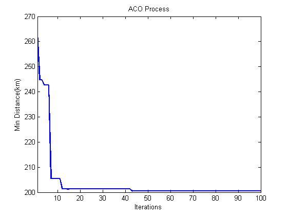
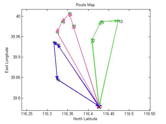
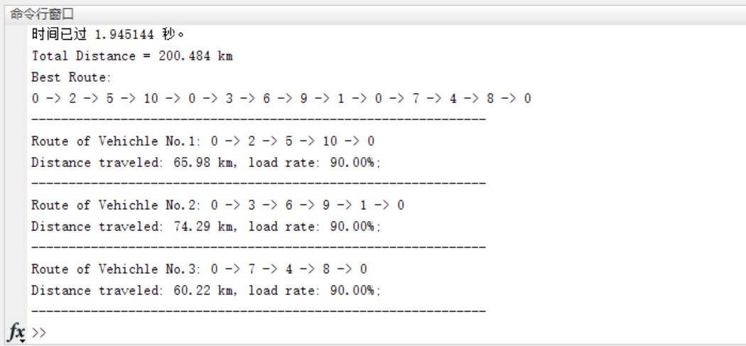
3, Operation results

4, Remarks

Version: 2014a