catalogue
1 genetic algorithm
Step 1: the setting of relevant parameters generally includes coding length L, population size M, number of iterations G, crossover rate Pc, mutation rate Pm, etc.
Step 2: the solution in the mathematical model cannot be directly used in the algorithm. The solution needs to be processed to construct the chromosome of the fitness function.
Step 3: M individuals are randomly generated to form the initial population Po, and the individuals are orderly distributed in the solution space. Each individual is a solution corresponding to the problem.
Step 4: calculate the fitness of each individual, and carry out selection and other operations in the population according to the fitness.
Step 5: according to the fitness of each individual, select individuals with high fitness for individual selection and other operations. The commonly used methods include roulette and so on.
Step 6: set the crossover rate Pc to control the crossover operation of the parent chromosome, and the crossed individual will enter the new species group instead of the parent.
Step 7: set the mutation rate Pm and control the mutation operation of the parent chromosome. Mutations can lead to the reappearance of genes that do not appear in the population or are eliminated in the selection process, and mutant individuals replace their parents into the new population.
Step 8: judge whether the updated population after the selection, crossover and mutation operations of the next iteration meets the termination conditions. If not, go back to step 4 for cyclic iteration; If it is satisfied, the algorithm will be stopped, and the maximum number of iterations is usually used as the termination criterion.
Step 9: decode the chromosome that meets the termination conditions to obtain the optimal solution of the problem. According to the above steps, we can know the basic process of genetic algorithm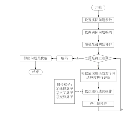
2 code display
clear
clc
close all
tic
%% use importdata This function reads the file
% shuju=importdata('cc101.txt');
load('cc101');
shuju=c101;
% bl=importdata('103.txt');
bl=3;
cap=60; %Maximum vehicle load
%% Extract data information
E=shuju(1,5); %Start time of distribution center time window
L=shuju(1,6); %End time of distribution center time window
zuobiao=shuju(:,2:3); %Coordinates of all points x and y
pszx=zuobiao(1:4,:);
customer=zuobiao(5:end,:); %Customer coordinates
cusnum=size(customer,1); %Number of customers
v_num=20; %Maximum number of vehicles used
demands=shuju(5:end,4); %requirement
a=shuju(5:end,5); %Customer time window start time[a[i],b[i]]
b=shuju(5:end,6); %End time of customer time window[a[i],b[i]]
s=shuju(5:end,7); %Customer service time
h=pdist(zuobiao);
dist=squareform(h);
% dist=load('dist.mat');
% dist=struct2cell(dist);
% dist=cell2mat(dist);
dist=dist./1000;%The distance matrix satisfies the triangular relationship and temporarily uses the distance to represent the cost c[i][j]=dist[i][j]
%% Genetic algorithm parameter setting
alpha=100000; %Penalty function coefficients for violating capacity constraints
belta=90;%Penalty function coefficient for violation of time window constraint
belta2=60;
chesu=20;
NIND=300; %Population size
MAXGEN=10; %Number of iterations
Pc=0.9; %Crossover probability
Pm=0.05; %Variation probability
GGAP=0.9; %generation gap(Generation gap)
N=cusnum+v_num-1; %Chromosome length=Number of customers+Maximum number of vehicles used-1
% N=cusnum;
%% Initialize population
% init_vc=init(cusnum,a,demands,cap);
dpszx = struct('ps',[], 'Chrom',[]);
dpszx.Chrom=InitPopCW(NIND,N,cusnum,a,demands,cap); %Construct initial solution
ps=pszxxz(dpszx.Chrom,cusnum);
%% Route and total distance of output random solution
disp('A random value in the initial population:')
[VC,NV,TD,violate_num,violate_cus]=decode(dpszx.Chrom(1,:),cusnum,cap,demands,a,b,L,s,dist,chesu,bl);
% [VC,NV]=cls(dpszx.Chrom(1,:),cusnum);
% [~,~,bsv]=violateTW(VC,a,b,s,L,dist,chesu,bl);
% disp(['Total distance:',num2str(TD)]);
disp(['Number of vehicles used:',num2str(NV),',Total vehicle distance:',num2str(TD)]);
disp('~~~~~~~~~~~~~~~~~~~~~~~~~~~~~~~~~~~~~~~~~~~~~~~~~~~~~~~~~~~~~~~~')
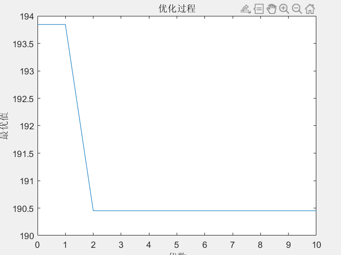
%% optimization
gen=1;
figure;
hold on;box on
xlim([0,MAXGEN])
title('Optimization process')
xlabel('Algebra')
ylabel('optimal value')
ObjV=calObj(dpszx.Chrom,cusnum,cap,demands,a,b,L,s,dist,alpha,belta,belta2,chesu,bl,ps); %Calculate the value of population objective function
preObjV=min(ObjV);
%%
while gen<=MAXGEN
%% Calculate fitness
ObjV=calObj(dpszx.Chrom,cusnum,cap,demands,a,b,L,s,dist,alpha,belta,belta2,chesu,bl,ps); %Calculate the value of population objective function
line([gen-1,gen],[preObjV,min(ObjV)]);pause(0.0001)%Drawing optimal function
preObjV=min(ObjV);
FitnV=Fitness(ObjV);
%% choice
[SelCh,psc]=Select(dpszx.Chrom,FitnV,GGAP,ps);
%% OX Cross operation
[SelCh,psc]=Recombin(SelCh,Pc,psc,cusnum);
%% variation
[SelCh,psc]=Mutate(SelCh,Pm,psc,cusnum);
%% New populations of reinsertion Progenies
[dpszx.Chrom,ps]=Reins(dpszx.Chrom,SelCh,ObjV,psc,ps);
%% Print current optimal solution
ObjV=calObj(dpszx.Chrom,cusnum,cap,demands,a,b,L,s,dist,alpha,belta,belta2,chesu,bl,ps); %Calculate the value of population objective function
[minObjV,minInd]=min(ObjV);
disp(['The first',num2str(gen),'Generation optimal solution:'])
[bestVC,bestNV,bestTD,best_vionum,best_viocus]=decode(dpszx.Chrom(minInd(1),:),cusnum,cap,demands,a,b,L,s,dist,chesu,bl);
disp(['Number of vehicles used:',num2str(bestNV),',Total vehicle distance:',num2str(bestTD)]);
fprintf('\n')
%% Update iterations
gen=gen+1 ;
end
%% Draw the road map of the optimal solution
ObjV=calObj(dpszx.Chrom,cusnum,cap,demands,a,b,L,s,dist,alpha,belta,belta2,chesu,bl,ps); %Calculate the value of population objective function
[minObjV,minInd]=min(ObjV);
%% Route and total distance of output optimal solution
disp('Optimal solution:')
bestChrom=dpszx.Chrom(minInd(1),:);
bestps=ps(minInd(1),:);
[bestVC,bestNV,bestTD,best_vionum,best_viocus]=decode(bestChrom,cusnum,cap,demands,a,b,L,s,dist,chesu,bl);
disp(['Number of vehicles used:',num2str(bestNV),',Total vehicle distance:',num2str(bestTD)]);
disp('-------------------------------------------------------------')
% [cost]=costFuction(bestVC,a,b,s,L,dist,demands,cap,alpha,belta,belta2,chesu,bl,);
%% Draw the final road map
draw_Best(bestVC,zuobiao,bestps);
% save c101.mat
% toc
3 simulation results
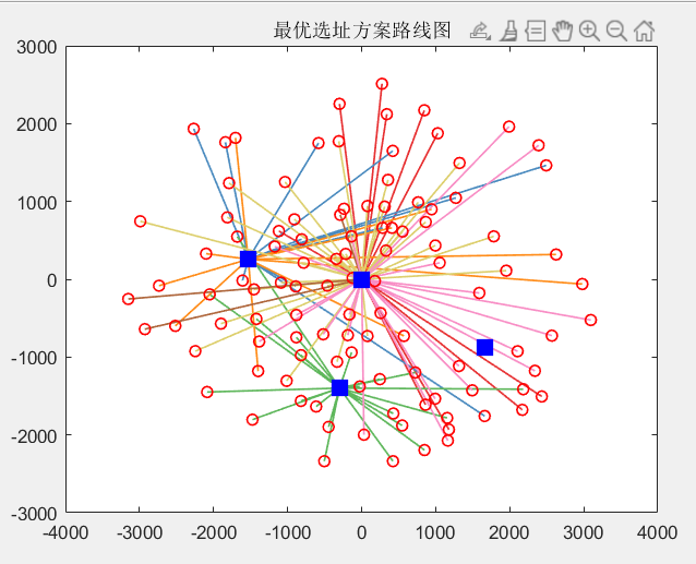

Site selection 1: 1 - > 29 - > 28 - > 27 - > 26 - > 25 - > 24 - > 23 - > 22 - > 21 - > 20 - > 1
Site selection 2: 4 - > 33 - > 43 - > 41 - > 40 - > 39 - > 38 - > 37 - > 36 - > 35 - > 34 - > 32 - > 4
Site selection 3: 2 - > 48 - > 62 - > 60 - > 58 - > 56 - > 55 - > 54 - > 53 - > 52 - > 51 - > 50 - > 49 - > 47 - > 76 - > 75 - > 74 - > 73 - > 72 - > 71 - > 70 - > 69 - > 2
Site selection 4: 4 - > 78 - > 90 - > 85 - > 84 - > 83 - > 82 - > 81 - > 80 - > 79 - > 77 - > 4
Site selection 5: 1 - > 92 - > 100 - > 105 - > 108 - > 107 - > 106 - > 104 - > 103 - > 101 - > 2 - > 14 - > 13 - > 12 - > 59 - > 99 - > 86 - > 57 - > 97 - > 96 - > 95 - > 93 - > 9 - > 8 - > 7 - > 5 - > 4 - > 3 - > 1 - > 91 - > 89 - > 88 - > 87 - > 1
Site selection 6:1 - > 16 - > 11 - > 10 - > 94 - > 1
Site selection 7: 1 - > 19 - > 18 - > 17 - > 15 - > 31 - > 30 - > 46 - > 98 - > 102 - > 6 - > 65 - > 64 - > 63 - > 61 - > 67 - > 68 - > 66 - > 45 - > 44 - > 42 - > 1
The first point is the selected distribution center (there are four alternative centers in the code)
Code download https://www.cnblogs.com/matlabxiao/p/14883637.html