Data set review
Firstly, the iris data set is reviewed, which provides 150 groups of iris data. Each group includes four input characteristics of iris: calyx length, calyx width, petal length and petal width. At the same time, the iris category corresponding to this group of characteristics is also given. Categories include dog iris, variegated iris and Virginia iris, which are represented by numbers 0, 1 and 2 respectively. The code for using this dataset is as follows:
from sklearn.datasets import load_iris
x_data = datasets.load_iris().data # Returns all input characteristics of iris dataset
y_data = datasets.load_iris().target # Return all tags of iris dataset
That is, export the data set from the sklearn package and assign the input feature to x_data variable, assign the corresponding label to y_data variable.
Program implementation
We only need three steps to realize iris classification with neural network:
(1) Prepare data, including data set reading and data set disorder, match the data of training set and test set into input feature and label pair, and generate train and test, that is, training set and test set that will never meet;
(2) Build the network and define all trainable parameters in the neural network;
(3) Optimize these trainable parameters, use the nested loop to obtain the partial derivative of the loss function loss to each trainable parameter in the with structure, and change these trainable parameters. In order to see the effect, the program can add each traversal data set to display the current accuracy, and draw the change curve of accuracy acc and loss function loss.
The complete code and analysis of the above parts are as follows:
(1) Dataset read in:
from sklearn.datasets import datasets
x_data = datasets.load_iris().data # Returns all input characteristics of iris dataset
y_data = datasets.load_iris().target # Return all tags of iris dataset
(2) Data set disorder:
np.random.seed(116) # Use the same seed to make the input features / labels correspond one by one
np.random.shuffle(x_data)
np.random.seed(116)
np.random.shuffle(y_data)
tf.random.set_seed(116)
(3) The data set is divided into training set and test set that will never meet:
x_train = x_data[:-30] #Intercept the data from 0 to the penultimate 30th as the training set
y_train = y_data[:-30]
x_test = x_data[-30:]#Intercept the test set from the last 30 to the last
y_test = y_data[-30:]
(4) Match [input feature, label] pairs and feed a small batch each time:
Feeding a batch is equivalent to training 32 lines of data each time, directly training two-dimensional data (different from the previous examples, our previous examples were based on one line of one-dimensional data).
train_db = tf.data.Dataset.from_tensor_slices((x_train, y_train)).batch(32)
test_db = tf.data.Dataset.from_tensor_slices((x_test, y_test)).batch(32)
(5) Define all trainable parameters in the neural network:
w1 = tf.Variable(tf.random.truncated_normal([ 4, 3 ], stddev=0.1, seed=1))
b1 = tf.Variable(tf.random.truncated_normal([ 3 ], stddev=0.1, seed=1))
On the premise of using only one layer of network, the definitions of w1 and b1 here are regular. Our input is 4 and the middle layer is 3, so w1 is usually in the matrix form of [4,3]. The middle layer is 3, so b1 is usually defined as 3.
(6) Nested loop iteration, with structure update parameter, display current loss:
for epoch in range(epoch): #Data set level iteration (how many times to calculate the whole training data)
 for step, (x_train, y_train) in enumerate(train_db): #batch level iteration
	 with tf.GradientTape() as tape: # Record gradient information
		y = tf.matmul(x_train, w1) + b1  # Neural network multiplication and addition operation
		y = tf.nn.softmax(y)  # Make the output y conform to the probability distribution (after this operation, it is the same order of magnitude as the single hot code, and the loss can be calculated by subtraction)
		y_ = tf.one_hot(y_train, depth=3)  # Convert the tag value to the unique hot code format to facilitate the calculation of loss and accuracy
		loss = tf.reduce_mean(tf.square(y_ - y))  # Use the mean square error loss function mse = mean(sum(y-out)^2)
		loss_all += loss.numpy()  # Accumulate the loss calculated by each step to provide data for the subsequent average of loss, so that the calculated loss is more accurate
	 grads = tape.gradient(loss, [ w1, b1 ]) #The partial derivatives of loss to w1 and b1 are obtained into an array. grads[0] is the partial derivative of loss to w1 and grads[1] is the partial derivative of loss to b1
	 w1.assign_sub(lr * grads[0]) #w1 self updating
 	 b1.assign_sub(lr * grads[1]) #b1 self updating
 print("Epoch {}, loss: {}".format(epoch, loss_all/4)) #The reason for dividing by 4 is that a batch needs to process 32 rows of data, while we have 128 rows of data. In this way, the second level loop, batch level iteration, needs to be carried out four times. Moreover, we require loss for each batch, and we have to accumulate the loss of the last batch for a total of 4 times, so we have to divide by 4
 train_loss_results.append(loss_all / 4)  # Average the loss of four step s and record it in this variable for the purpose of printing the loss curve below
This code describes softmax and one in the previous article_ The actual application scenario of hot uses softmax to calculate y_ Convert to the form of probability distribution and the one of y of the original label_ The mean square error is calculated by subtraction in hot form
(7) Calculate the accuracy rate of the current parameter after forward propagation, and display the current accuracy rate acc:
 # Test part
    # total_correct is the number of samples of the prediction pair, total_number is the total number of samples tested, and both variables are initialized to 0
    total_correct, total_number = 0, 0
    for x_test, y_test in test_db:
        # The trained parameters of W1 and B1 are used for prediction
        y = tf.matmul(x_test, w1) + b1
        # The predicted value is converted into the form of probability distribution
        y = tf.nn.softmax(y)
        # Returns the index of the maximum value in y, that is, the classification of the prediction
        pred = tf.argmax(y, axis=1)
        # Convert pred to y_ Data type of test
        pred = tf.cast(pred, dtype=y_test.dtype)
        # If the classification is correct, correct=1, otherwise it is 0, and the result of bool type is converted to int type
        correct = tf.cast(tf.equal(pred, y_test), dtype=tf.int32)
        # Add up the correct number of each batch
        correct = tf.reduce_sum(correct)
        # Add up the number of correct in all batch es
        total_correct += int(correct)
        # total_number is the total number of samples tested, which is X_ The number of rows of test. shape[0] returns the number of rows of variables tested each time
        total_number += x_test.shape[0]
    # The total accuracy is equal to total_correct/total_number
    acc = total_correct / total_number
    test_acc.append(acc) #The purpose is to print the acc curve below
    print("Test_acc:", acc)
    print("--------------------------")
(8) acc / loss visualization:
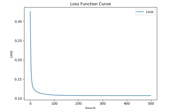
plt.title('Loss Function Curve')  # Picture title
plt.xlabel('Epoch')  # x-axis variable name
plt.ylabel('Loss')  # y-axis variable name
plt.plot(train_loss_results, label="$Loss$")  # Draw trian point by point_ Loss_ The results value and connect, and the connection icon is Loss
plt.legend()  # Draw a curve Icon
plt.show()  # Draw an image
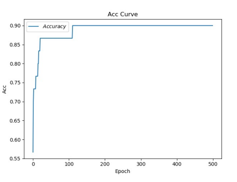
plt.title('Acc Curve')  # Picture title
plt.xlabel('Epoch')  # x-axis variable name
plt.ylabel('Acc')  # y-axis variable name
plt.plot(test_acc, label="$Accuracy$")  # Draw the test point by point_ ACC value and connect. The connection icon is Accuracy
plt.legend()
plt.show()