1, Introduction

1 overview of genetic algorithm
Genetic Algorithm (GA) is a part of evolutionary computation. It is a computational model that simulates the biological evolution process of Darwin's genetic selection and natural elimination. It is a method to search the optimal solution by simulating the natural evolution process. The algorithm is simple, universal, robust and suitable for parallel processing.

2 characteristics and application of genetic algorithm
Genetic algorithm is a kind of robust search algorithm that can be used for complex system optimization. Compared with the traditional optimization algorithm, it has the following characteristics:
(1) Take the code of decision variable as the operation object. Traditional optimization algorithms often directly use the actual value of decision variables itself for optimization calculation, but genetic algorithm uses some form of coding of decision variables as the operation object. This coding method of decision variables enables us to learn from the concepts of chromosome and gene in biology in optimization calculation, imitate the genetic and evolutionary incentives of organisms in nature, and easily apply genetic operators.
(2) Directly take fitness as search information. The traditional optimization algorithm not only needs to use the value of the objective function, but also the search process is often constrained by the continuity of the objective function. It may also need to meet the requirement that "the derivative of the objective function must exist" to determine the search direction. Genetic algorithm only uses the fitness function value transformed from the objective function value to determine the further search range, without other auxiliary information such as the derivative value of the objective function. Directly using the objective function value or individual fitness value can also focus the search range into the search space with higher fitness, so as to improve the search efficiency.
(3) Using the search information of multiple points has implicit parallelism. The traditional optimization algorithm is often an iterative search process starting from an initial point in the solution space. The search information provided by a single point is not much, so the search efficiency is not high, and it may fall into local optimal solution and stop; Genetic algorithm starts the search process of the optimal solution from the initial population composed of many individuals, rather than from a single individual. The, selection, crossover, mutation and other operations on the initial population produce a new generation of population, including a lot of population information. This information can avoid searching some unnecessary points, so as to avoid falling into local optimization and gradually approach the global optimal solution.
(4) Use probabilistic search instead of deterministic rules. Traditional optimization algorithms often use deterministic search methods. The transfer from one search point to another has a certain transfer direction and transfer relationship. This certainty may make the search less than the optimal store, which limits the application scope of the algorithm. Genetic algorithm is an adaptive search technology. Its selection, crossover, mutation and other operations are carried out in a probabilistic way, which increases the flexibility of the search process, and can converge to the optimal solution with a large probability. It has a good ability of global optimization. However, crossover probability, mutation probability and other parameters will also affect the search results and search efficiency of the algorithm, so how to select the parameters of genetic algorithm is a more important problem in its application.
To sum up, because the overall search strategy and optimization search mode of genetic algorithm do not rely on gradient information or other auxiliary knowledge, and only need to solve the objective function and corresponding fitness function affecting the search direction, genetic algorithm provides a general framework for solving complex system problems. It does not depend on the specific field of the problem and has strong robustness to the types of problems, so it is widely used in various fields, including function optimization, combinatorial optimization, production scheduling problem and automatic control
, robotics, image processing (image restoration, image edge feature extraction...), artificial life, genetic programming, machine learning.

3 basic flow and implementation technology of genetic algorithm
Simple genetic algorithms (SGA) only uses three genetic operators: selection operator, crossover operator and mutation operator. The evolution process is simple and is the basis of other genetic algorithms.

3.1 basic flow of genetic algorithm
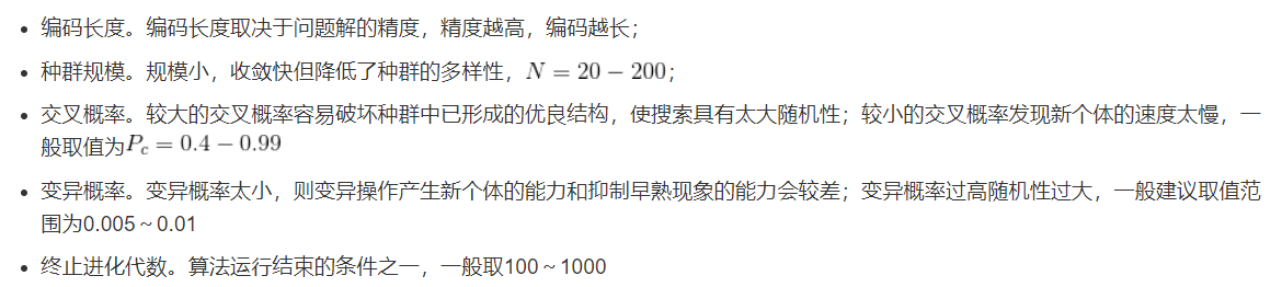
Generating a number of initial groups encoded by a certain length (the length is related to the accuracy of the problem to be solved) in a random manner;
Each individual is evaluated by fitness function. Individuals with high fitness value are selected to participate in genetic operation, and individuals with low fitness are eliminated;
A new generation of population is formed by the collection of individuals through genetic operation (replication, crossover and mutation) until the stopping criterion is met (evolutionary algebra gen > =?);
The best realized individual in the offspring is taken as the execution result of genetic algorithm.

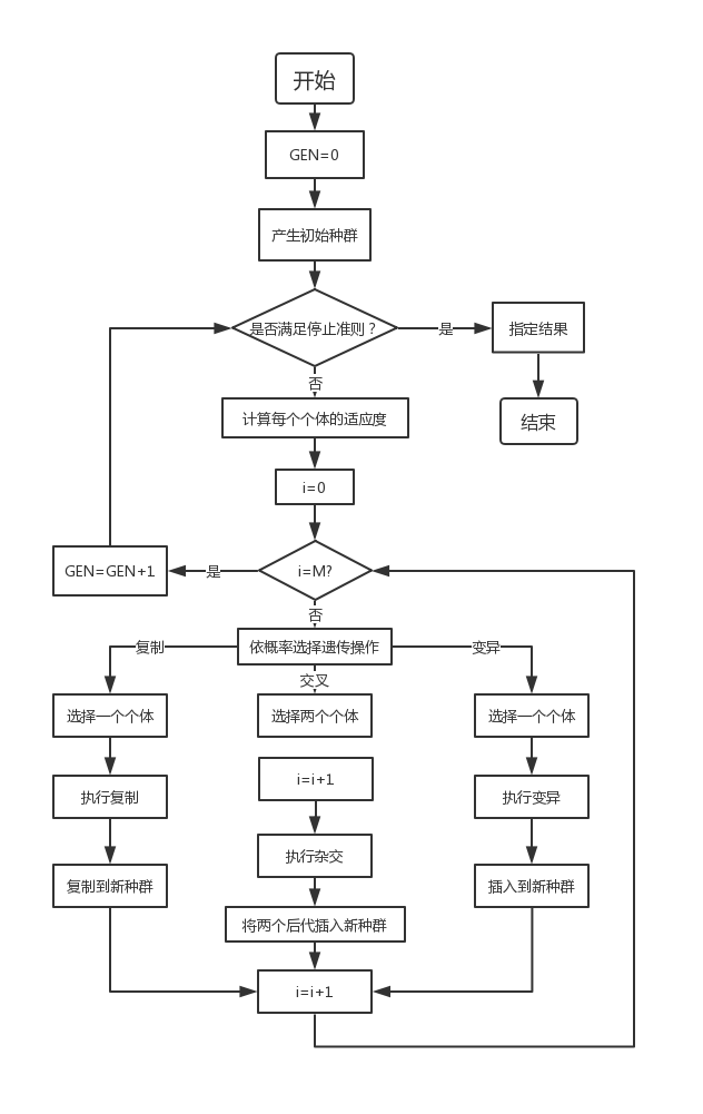
Where GEN is the current algebra; M is the population size, and i represents the population number.

3.2 implementation technology of genetic algorithm
Basic genetic algorithm (SGA) consists of coding, fitness function, genetic operators (selection, crossover, mutation) and operating parameters.
3.2.1 coding
(1) Binary coding
The length of binary coded string is related to the accuracy of the problem. It is necessary to ensure that every individual in the solution space can be encoded.
Advantages: the operation of encoding and decoding is simple, and the inheritance and crossover are easy to realize
Disadvantages: large length
(2) Other coding methods
Gray code, floating point code, symbol code, multi parameter code, etc
3.2.2 fitness function
The fitness function should effectively reflect the gap between each chromosome and the chromosome of the optimal solution of the problem.
3.2.3 selection operator

3.2.4 crossover operator
Cross operation refers to the exchange of some genes between two paired chromosomes in some way, so as to form two new individuals; Crossover operation is an important feature that distinguishes genetic algorithm from other evolutionary algorithms. It is the main method to generate new individuals. Before crossing, individuals in the group need to be paired. Generally, the principle of random pairing is adopted.
Common crossing methods:
Single point intersection
Double point crossing (multi-point crossing, the more crossing points, the greater the possibility of individual structure damage, and multi-point crossing is generally not adopted)
Uniform crossing
Arithmetic Crossover
3.2.5 mutation operator
Mutation operation in genetic algorithm refers to replacing the gene value of some loci in the individual chromosome coding string with other alleles of the locus, so as to form a new individual.

In terms of the ability to generate new individuals in the operation process of genetic algorithm, crossover operation is the main method to generate new individuals, which determines the global search ability of genetic algorithm; Mutation is only an auxiliary method to generate new individuals, but it is also an essential operation step, which determines the local search ability of genetic algorithm. The combination of crossover operator and mutation operator completes the global search and local search of the search space, so that the genetic algorithm can complete the optimization process of the optimization problem with good search performance.

3.2.6 operating parameters

4 basic principle of genetic algorithm
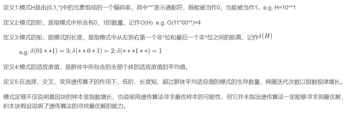
4.1 mode theorem

4.2 building block assumptions
Patterns with low order, short definition length and fitness value higher than the average fitness value of the population are called gene blocks or building blocks.
Building block hypothesis: individual gene blocks can be spliced together through the action of genetic operators such as selection, crossover and mutation to form individual coding strings with higher fitness.
The building block hypothesis illustrates the basic idea of solving various problems with genetic algorithm, that is, better solutions can be produced by directly splicing the building blocks together.

2, Source code

clc %Clear command line window
clear %Deletes all variables from the current workspace and frees them from system memory
close all %Delete all windows whose handles are not hidden
tic % Save current time
%% GA-PSO Algorithm solving DVRP
%Input:
%City           Longitude and latitude of demand point
%Distance       Distance matrix
%Travelcon      Travel constraint
%NIND           Population number
%MAXGEN         Inherited to the third MAXGEN Time substitution program stop

%Output:
%Gbest          Shortest path
%GbestDistance	Shortest path length

%% Load data
load('City.mat')	      %The longitude and latitude of the demand point is used to draw the actual path XY coordinate
load('Distance.mat')	  %Distance matrix
load('Travelcon.mat')	  %Travel constraint

%% Initialize problem parameters
CityNum=size(City,1)-1; %Number of demand points

%% Initialization algorithm parameters
NIND=60; %Number of particles
MAXGEN=100; %Maximum number of iterations

%% 0 matrix initialized for pre allocation of memory
Population = zeros(NIND,CityNum*2+1); %Pre allocated memory for storing population data
PopDistance = zeros(NIND,1); %Pre allocate matrix memory
GbestDisByGen = zeros(MAXGEN,1); %Pre allocate matrix memory

for i = 1:NIND
    %% Initialize each particle
    Population(i,:)=InitPop(CityNum,Distance,Travelcon); %Random generation TSP route
    
    %% Calculate path length
    PopDistance(i) = CalcDis(Population(i,:),Distance,Travelcon); % Calculate path length
end

%% storage Pbest data
Pbest = Population; % initialization Pbest For the current particle collection
PbestDistance = PopDistance; % initialization Pbest The objective function value of is the objective function value of the current particle set

%% storage Gbest data
[mindis,index] = min(PbestDistance); %get Pbest in
Gbest = Pbest(index,:); % initial Gbest particle
GbestDistance = mindis; % initial Gbest Objective function value of particle

%% Start iteration
gen=1;

while gen <= MAXGEN
    %% Update per particle
    for i=1:NIND
        %% Particles and Pbest overlapping
        Population(i,2:end-1)=Crossover(Population(i,2:end-1),Pbest(i,2:end-1)); %overlapping
        
        % If the length of the new path becomes shorter, record to Pbest
        PopDistance(i) = CalcDis(Population(i,:),Distance,Travelcon); %Calculate distance
        if PopDistance(i) < PbestDistance(i) %If the length of the new path becomes shorter
            Pbest(i,:)=Population(i,:); %to update Pbest
            PbestDistance(i)=PopDistance(i); %to update Pbest distance
        end
        
        %% according to Pbest to update Gbest
        [mindis,index] = min(PbestDistance); %find Pbest Medium shortest distance

        if mindis < GbestDistance %if Pbest The shortest distance in is less than Gbest distance
            Gbest = Pbest(index,:); %to update Gbest
            GbestDistance = mindis; %to update Gbest distance
        end
        
        %% Particles and Gbest overlapping
        Population(i,2:end-1)=Crossover(Population(i,2:end-1),Gbest(2:end-1));
        
        % If the length of the new path becomes shorter, record to Pbest
        PopDistance(i) = CalcDis(Population(i,:),Distance,Travelcon); %Calculate distance
        if PopDistance(i) < PbestDistance(i) %If the length of the new path becomes shorter
            Pbest(i,:)=Population(i,:); %to update Pbest
            PbestDistance(i)=PopDistance(i); %to update Pbest distance
        end
        function a=Crossover(a,b)
%% PMX Method crossover
%Input:
%a  Path represented by particles
%b  Path represented by individual optimal particle

%Output:
%a	The path represented by the crossed particles

L=length(a); %Obtain parental chromosome length
r1=unidrnd(L); %In 1~L Select an integer at random
r2=unidrnd(L); %In 1~L Select an integer at random

s=min([r1,r2]); %The starting point is a smaller value
e=max([r1,r2]); %The end point is a larger value

b0=b(s:e); %For last insertion

aa=a(s:e); %Used to check for duplicate elements
bb=b(s:e); %Used to check for duplicate elements

a(s:e)=[];     %After removing the intersection, the following elements will move forward

outlen=length(a); %After removing the intersection,  a，b Length of   length outside cross section
inlen=e-s+1;      %Length of cross section  length inside cross section 

for i=1:inlen     %Remove the same elements from the intersection
	for j=1:inlen
		if aa(i)==bb(j) %If there are the same elements up and down in the intersection
			aa(i)=0; %delete
			bb(j)=0;
			break  %  break Can guarantee the final aa and bb Same length and no duplicate elements
		end
	end
end
function ttlDistance=CalcDis(route,Distance,Travelcon)
%% Calculate the path length fitness function of each individual  
%Input:
%route          Path represented by a particle
%Distance       Distance matrix between two cities
%Travelcon     Travel constraint

%Output:
%ttlDistance	Population individual path distance

%Related data initialization
DisTraveled=0;  % The distance the car has traveled
Dis=0; %The total distance of all vehicles in this scheme

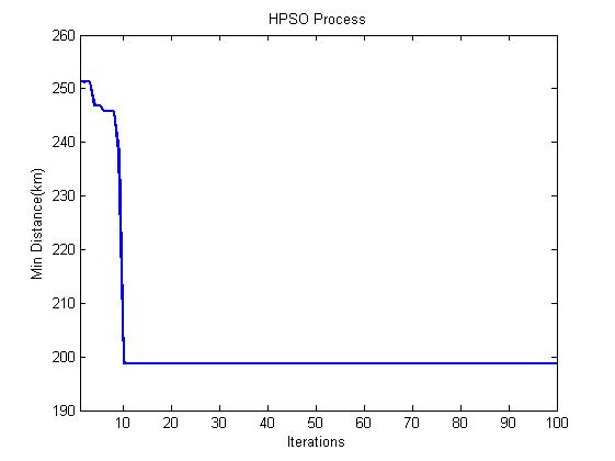
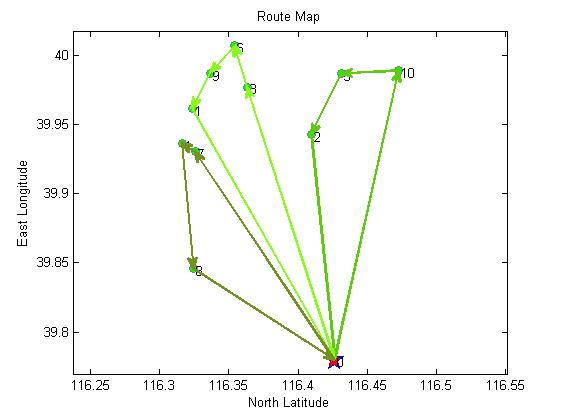
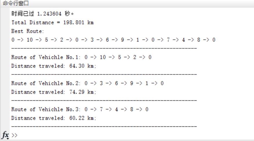
3, Operation results

4, Remarks

Version: 2014a