The time distributed layer is a sequence rather than a single value that needs to be returned by the LSTM layer in the Keras interface.
What is the time distributed layer
The added complexity is the TimeDistributed layer (and the previous TimeDistributedDense layer), which is mysteriously described as a layer wrapper that allows us to apply a layer to each time slice of input.
How and when should this wrapper be used with LSTM?
For example, TimeDistributedDense applies the same sense operation to each time step of the 3D tensor.
If you already know the purpose of the TimeDistributed layer and when to use it, it makes sense, but it's not helpful for beginners at all.
Sequential learning problem
We will use a simple sequence learning problem to demonstrate the TimeDistributed layer.
In this problem, the sequence [0.0, 0.2, 0.4, 0.6, 0.8] will be given one item at a time as input, and must be returned one item at a time as output in turn.
Think of it as learning a simple echo program. We give 0.0 as input, and we want to see 0.0 as output, repeating for each item in the sequence.
We can directly generate this sequence as follows:
from numpy import array
length = 5
seq = array([i/float(length) for i in range(length)])
print(seq)
Run this example to print the generated sequence:
[ 0. 0.2 0.4 0.6 0.8]
The example is configurable, and you can play longer / shorter sequences yourself later if you like. Let me know your results in the comments.
LSTM one-to-one for sequence prediction
Before we further study, it is important to prove that this sequential learning problem can be segmented learning.
That is, we can reconstruct the problem into a data set of input-output pairs for each item in the sequence. Given 0, the network should output 0, given 0.2, the network must output 0.2, and so on.
This is the simplest expression of the problem. We need to split the sequence into input-output pairs, predict the sequence step by step and collect it outside the network.
The input and output pairs are as follows:
X, 	y
0.0,	0.0
0.2,	0.2
0.4,	0.4
0.6,	0.6
0.8,	0.8
The input of LSTM must be three-dimensional. We can reshape the 2D sequence into a 3D sequence with 5 samples, 1 time step and 1 feature. We define the output as five samples with one feature.
X = seq.reshape(5, 1, 1)
y = seq.reshape(5, 1)
We define the network model as having one input and one time step. The first hidden layer will be an LSTM with 5 cells. The output layer is a fully connected layer with one output.
The model will be fitted with efficient ADAM optimization algorithm and mean square error loss function.
The batch size is set to the number of samples in the epoch to avoid having to Staten the LSTM and manually manage the state reset, although this can be easily done to update the weight after each sample is displayed to the network.
The complete code list is as follows:
from numpy import array
from keras.models import Sequential
from keras.layers import Dense
from keras.layers import LSTM
# Prepare sequence data
length = 5
seq = array([i/float(length) for i in range(length)])
X = seq.reshape(len(seq), 1, 1)
y = seq.reshape(len(seq), 1)
# Define LSTM configuration
n_neurons = length
n_batch = length
n_epoch = 1000
# Create LSTM
model = Sequential()
model.add(LSTM(n_neurons, input_shape=(1, 1)))
model.add(Dense(1))
model.compile(loss='mean_squared_error', optimizer='adam')
print(model.summary())
# Training LSTM
model.fit(X, y, epochs=n_epoch, batch_size=n_batch, verbose=2)
# assessment
result = model.predict(X, batch_size=n_batch, verbose=0)
for value in result:
	print('%.1f' % value)
The running example first prints the structure of the configuration network.
We can see that the LSTM layer has 140 parameters. This is calculated based on the number of inputs (1) and the number of outputs (5 for 5 cells in the hidden layer), as follows:
n = 4 * ((inputs + 1) * outputs + outputs^2)
n = 4 * ((1 + 1) * 5 + 5^2)
n = 4 * 35
n = 140
We can also see that there are only six parameters in the full connection layer, which are the number of inputs (five represent the five inputs of the previous layer), the number of outputs (one represents one neuron in this layer) and bias.
n = inputs * outputs + outputs
n = 5 * 1 + 1
n = 6
_________________________________________________________________
Layer (type)                 Output Shape              Param #
=================================================================
lstm_1 (LSTM)                (None, 1, 5)              140
_________________________________________________________________
dense_1 (Dense)              (None, 1, 1)              6
=================================================================
Total params: 146.0
Trainable params: 146
Non-trainable params: 0.0
_________________________________________________________________
The network correctly learns the prediction problem.
0.0
0.2
0.4
0.6
0.8
LSTM many to one for sequence prediction (no TimeDistributed)
In this section, we developed an LSTM to output all sequences at once, although there is no TimeDistributed wrapper layer.
The input of LSTM must be three-dimensional. We can reshape the 2D sequence into a 3D sequence with 1 sample, 5 time steps and 1 feature. We define the output as one sample with five characteristics.
X = seq.reshape(1, 5, 1)
y = seq.reshape(1, 5)
Immediately, you can see that the problem definition must be slightly adjusted to support a sequence prediction network without a TimeDistributed wrapper. Specifically, output a vector instead of building an output sequence step by step. The differences may sound subtle, but it's important to understand the role of the TimeDistributed wrapper.
We define the model as an input with five time steps. The first hidden layer will be an LSTM with 5 cells. The output layer is a fully connected layer with five neurons.
# Create LSTM
model = Sequential()
model.add(LSTM(5, input_shape=(5, 1)))
model.add(Dense(length))
model.compile(loss='mean_squared_error', optimizer='adam')
print(model.summary())
Next, we only fit the model with 500 periods and batch size of 1 for a single sample in the training data set.
# Training LSTM
model.fit(X, y, epochs=500, batch_size=1, verbose=2)
Put all this together, a complete code listing is provided below.
from numpy import array
from keras.models import Sequential
from keras.layers import Dense
from keras.layers import LSTM
# Prepare sequence data
length = 5
seq = array([i/float(length) for i in range(length)])
X = seq.reshape(1, length, 1)
y = seq.reshape(1, length)
# Define LSTM configuration
n_neurons = length
n_batch = 1
n_epoch = 500
# Create LSTM
model = Sequential()
model.add(LSTM(n_neurons, input_shape=(length, 1)))
model.add(Dense(length))
model.compile(loss='mean_squared_error', optimizer='adam')
print(model.summary())
# Training LSTM
model.fit(X, y, epochs=n_epoch, batch_size=n_batch, verbose=2)
# assessment
result = model.predict(X, batch_size=n_batch, verbose=0)
for value in result[0,:]:
	print('%.1f' % value)
Running this example first prints a summary of the configured network.
We can see that the LSTM layer has 140 parameters as in the previous section.
LSTM cells have been weakened. Each cell will output a value and provide a vector containing five values as the input of the full connection layer. The time dimension or sequence information has been discarded and collapsed into a vector of 5 values.
We can see that the fully connected output layer has five inputs and five values are expected to be output. We can calculate the 30 weights to be learned as follows:
n = inputs * outputs + outputs
n = 5 * 5 + 5
n = 30
The network summary report is as follows:
_________________________________________________________________
Layer (type)                 Output Shape              Param #
=================================================================
lstm_1 (LSTM)                (None, 5)                 140
_________________________________________________________________
dense_1 (Dense)              (None, 5)                 30
=================================================================
Total params: 170.0
Trainable params: 170
Non-trainable params: 0.0
_________________________________________________________________
The model is fitted and the loss information is printed before the prediction sequence is finally determined and printed.
The sequence is reproduced correctly, but gradually as a single segment rather than through input data. We may use the sense layer as the first hidden layer instead of the LSTM, because this use of the LSTM does not make full use of their full sequence learning and processing capabilities.
0.0
0.2
0.4
0.6
0.8
LSTM many to many for sequence prediction (using TimeDistributed)
In this section, we will use the TimeDistributed layer to process the output from the LSTM hidden layer.
There are two key points to keep in mind when using TimeDistributed wrapper layers:
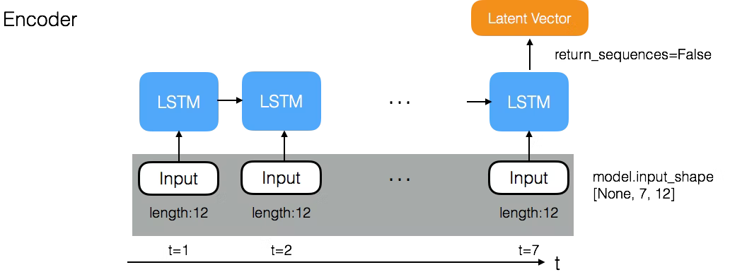
Input must be (at least) 3D. This usually means that you need to configure the last LSTM layer before the dense layer of the TimeDistributed package to return the sequence (for example, set the "return_sequences" parameter to "True").
The output will be 3D. This means that if the density layer of your TimeDistributed package is your output layer and you are predicting a sequence, you need to resize the y array to a 3D vector.
We can define the output shape as having 1 sample, 5 time steps and 1 feature, just like the input sequence, as follows:
y = seq.reshape(1, length, 1)
We can define the LSTM hidden layer to return sequences instead of individual values by setting the "return_sequences" parameter to true.
model.add(LSTM(n_neurons, input_shape=(length, 1), return_sequences=True))
This has the effect that each LSTM unit returns a sequence of five outputs, one for each time step in the input data, rather than a single output value in the previous example.
We can also wrap a fully connected sense layer with a single output using TimeDistributed on the output layer.
model.add(TimeDistributed(Dense(1)))
A single output value in the output layer is the key. It emphasizes that we intend to output a time step from the sequence for each time step in the input. As it happens, we will process five time steps of the input sequence at once.
TimeDistributed implements this technique by applying the same density layer (the same weight) to the LSTM output one time step at a time. In this way, only one output layer needs to be connected to each LSTM unit (plus a bias).
For this reason, it is necessary to increase the number of training periods to solve the small network capacity. I doubled it from 500 to 1000 to match the first one-to-one example.
Put these together, a complete code listing is provided below.
from numpy import array
from keras.models import Sequential
from keras.layers import Dense
from keras.layers import TimeDistributed
from keras.layers import LSTM
# Prepare sequence data
length = 5
seq = array([i/float(length) for i in range(length)])
X = seq.reshape(1, length, 1)
y = seq.reshape(1, length, 1)
# Define LSTM configuration
n_neurons = length
n_batch = 1
n_epoch = 1000
# Create LSTM
model = Sequential()
model.add(LSTM(n_neurons, input_shape=(length, 1), return_sequences=True))
model.add(TimeDistributed(Dense(1)))
model.compile(loss='mean_squared_error', optimizer='adam')
print(model.summary())
# Training LSTM
model.fit(X, y, epochs=n_epoch, batch_size=n_batch, verbose=2)
# assessment
result = model.predict(X, batch_size=n_batch, verbose=0)
for value in result[0,:,0]:
	print('%.1f' % value)
Running the example, we can see the configured network structure.
We can see that, as in the previous example, we have 140 parameters in the LSTM hidden layer.
The fully connected output layer is a very different story. In fact, it exactly matches the one-to-one example. A neuron has a weight for each LSTM unit in the previous layer, plus a weight for bias input.
There are two important things:
It allows the problem to be constructed and learned in a defined way, that is, one input to one output, so that the internal process of each time step remains independent.
Simplify the network by requiring less weight so that only one time step is processed at a time.
A simpler full connection layer is applied to each time step in the sequence provided by the previous layer to build the output sequence.
_________________________________________________________________
Layer (type)                 Output Shape              Param #
=================================================================
lstm_1 (LSTM)                (None, 5, 5)              140
_________________________________________________________________
time_distributed_1 (TimeDist (None, 5, 1)              6
=================================================================
Total params: 146.0
Trainable params: 146
Non-trainable params: 0.0
_________________________________________________________________
Similarly, e-learning sequence.
0.0
0.2
0.4
0.6
0.8
In the first example, we can see the framework of the problem with the time step and TimeDistributed layer as a more compact way to implement one-to-one networks. On a larger scale, it may even be more effective (in terms of space or time).