Scikit learn nanny level introductory tutorial

Scikit learn is a well-known Python machine learning library, which is widely used in data science fields such as statistical analysis and machine learning modeling.

• Modeling invincible: users can realize various supervised and unsupervised learning models through scikit learn
• Various functions: at the same time, using sklearn can also carry out data preprocessing, feature engineering, data set segmentation, model evaluation and so on
• Rich data: rich data sets are built in, such as Titanic, iris, etc. data is no longer worrying

This article introduces the use of scikit learn in a concise way. For more details, please refer to the official website:

1. Use of built-in dataset
2. Data set segmentation
3. Data normalization and standardization
4. Type code
5. Modeling 6

Scikit learn uses God map

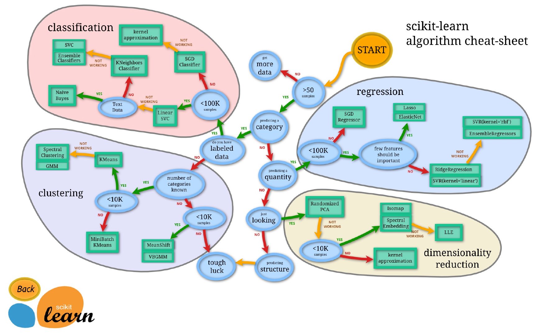
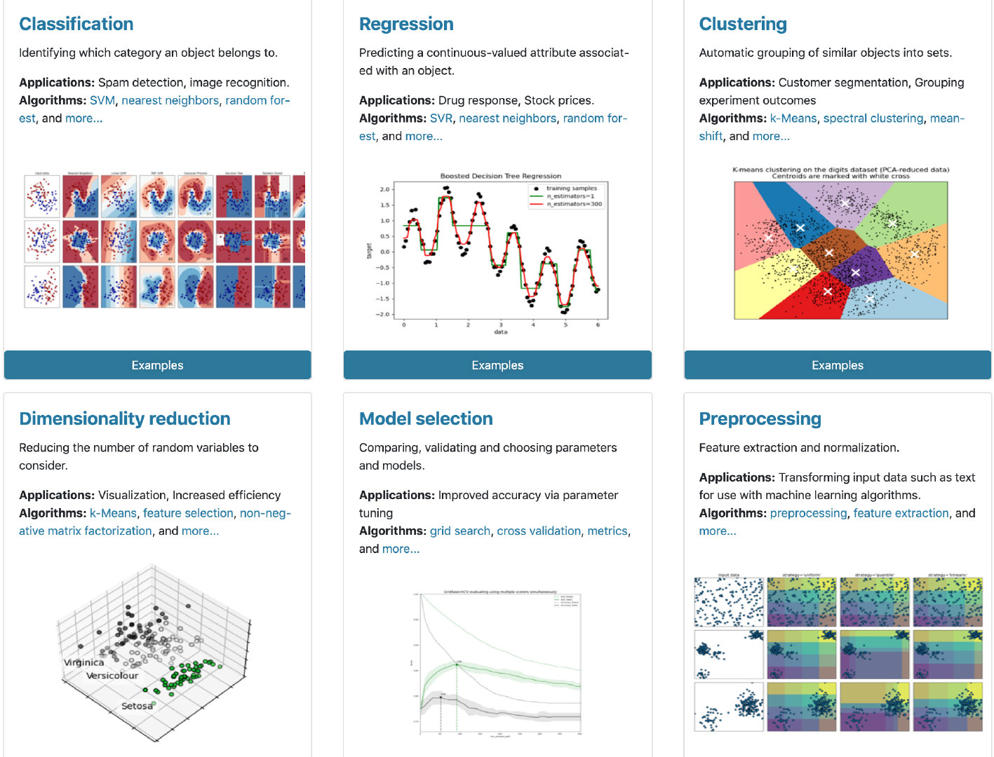
The following figure is provided on the official website. Starting from the size of the sample size, it summarizes the use of scikit learn in four aspects: regression, classification, clustering and data dimensionality reduction:

https://scikit-learn.org/stable/tutorial/machine_learning_map/index.html

install

For the installation of scikit learn, it is recommended to use anaconda for installation without worrying about various configuration and environmental problems. Of course, you can also directly install pip:

pip install scikit-learn

Dataset generation

sklearn has built-in some excellent data sets, such as Iris data, house price data, Titanic data, etc.

import pandas as pd
import numpy as np

import sklearn 
from sklearn import datasets  # Import dataset

Classified data iris data

# iris data
iris = datasets.load_iris()
type(iris)

sklearn.utils.Bunch

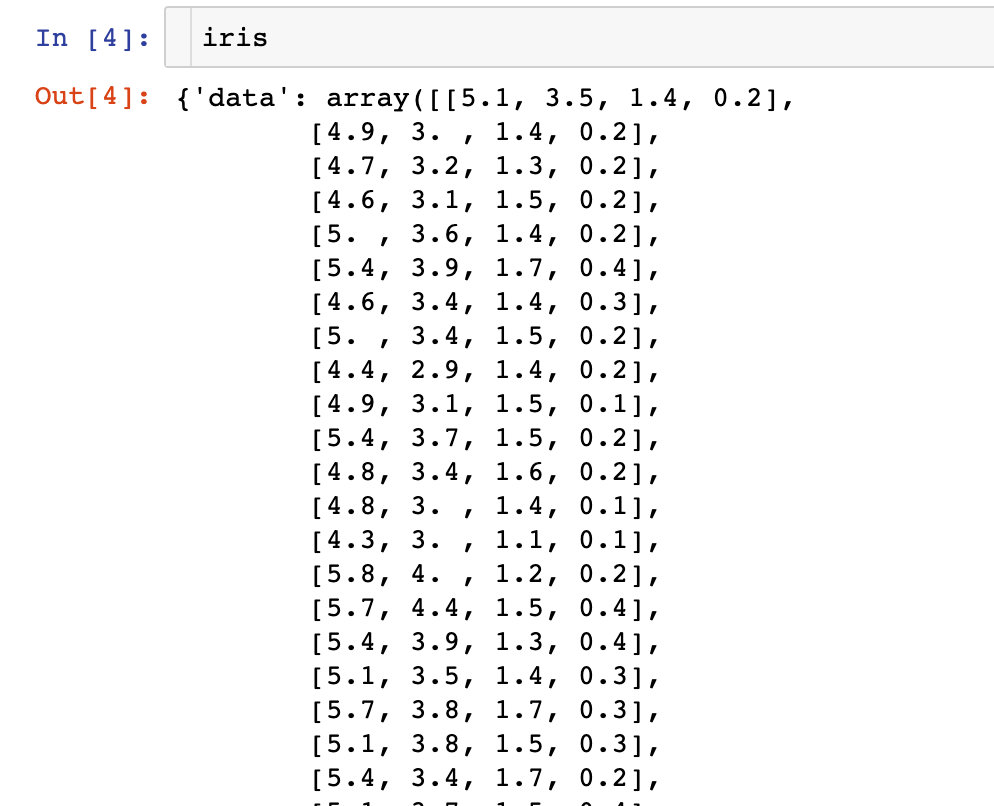
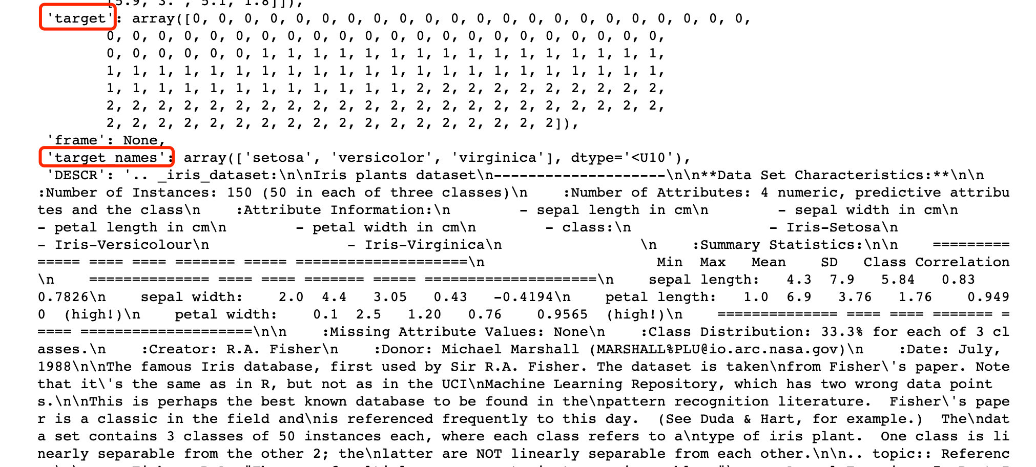
What is iris data like? Each built-in data contains a lot of information

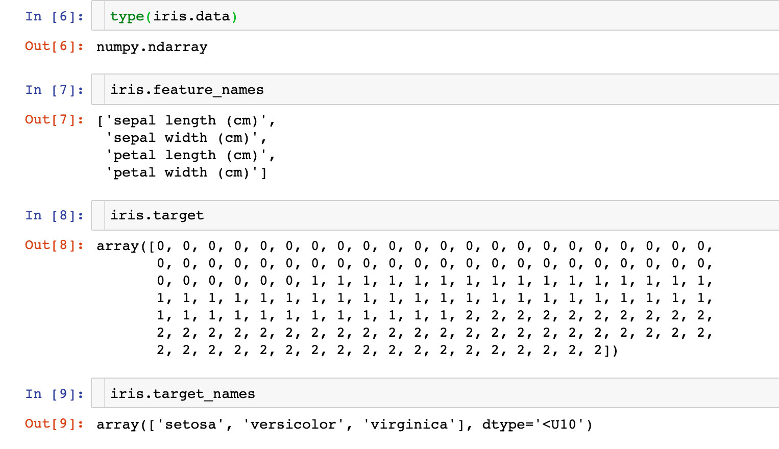
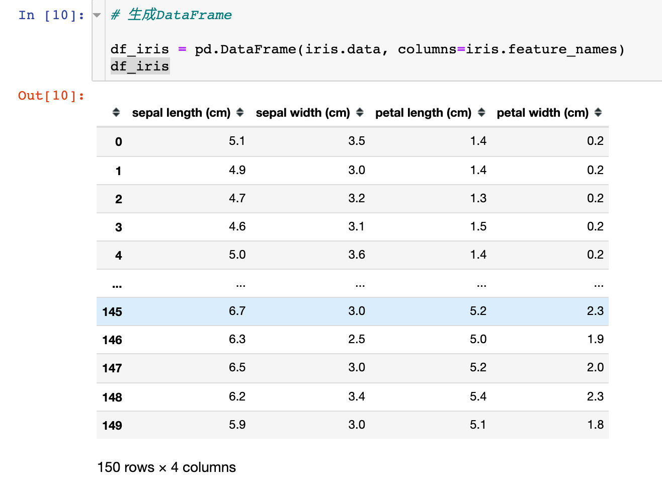
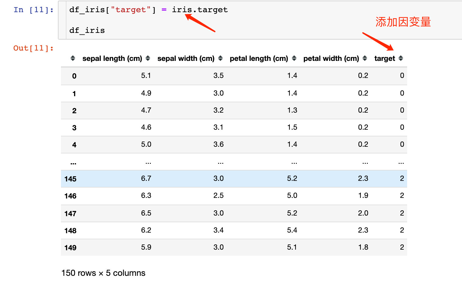
The above data can be generated into the DataFrame we want to see, and dependent variables can be added:

Regression data - Boston house prices

[external link image transfer failed. The source station may have anti-theft chain mechanism. It is recommended to save the image and upload it directly (img-de0fuhf4-1643120482)( https://tva1.sinaimg.cn/large/008i3skNly1gy91s2w95wj31ak0pqdlw.jpg )]

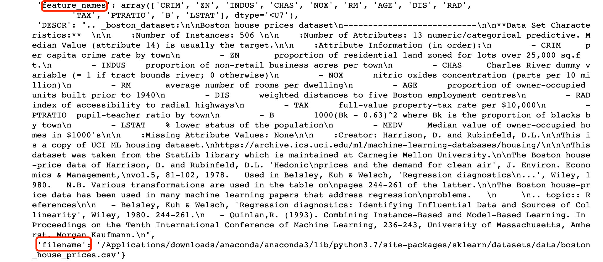
Attributes we focus on:

• data
• target,target_names
• feature_names
• filename

DataFrame can also be generated:

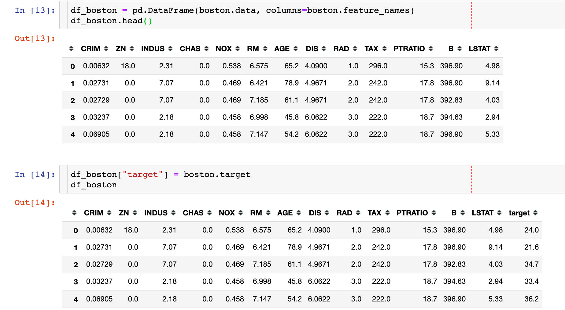
Three ways to generate data

Mode 1

#Call module
from sklearn.datasets import load_iris
data = load_iris()

#Import data and labels
data_X = data.data
data_y = data.target 

Mode 2

from sklearn import datasets
loaded_data = datasets.load_iris()  # Properties of the imported dataset

#Import sample data
data_X = loaded_data.data
# Import label
data_y = loaded_data.target

Mode 3

# Direct return
data_X, data_y = load_iris(return_X_y=True)

Data set Usage Summary

from sklearn import datasets  # Import library

boston = datasets.load_boston()  # Import Boston house price data
print(boston.keys())  # View key (attribute) [data','target','feature_names','DESCR', 'filename'] 
print(boston.data.shape,boston.target.shape)  # View the shape of the data 
print(boston.feature_names)  # See what features 
print(boston.DESCR)  # described dataset description information 
print(boston.filename)  # File path 

Data segmentation

# Import module
from sklearn.model_selection import train_test_split
# It is divided into training set and test set data
X_train, X_test, y_train, y_test = train_test_split(
  data_X, 
  data_y, 
  test_size=0.2,
  random_state=111
)

# 150*0.8=120
len(X_train)

Data standardization and normalization

from sklearn.preprocessing import StandardScaler  # Standardization
from sklearn.preprocessing import MinMaxScaler  # normalization

# Standardization
ss = StandardScaler()
X_scaled = ss.fit_transform(X_train)  # Incoming data to be standardized

# normalization
mm = MinMaxScaler()
X_scaled = mm.fit_transform(X_train)

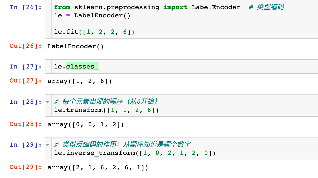
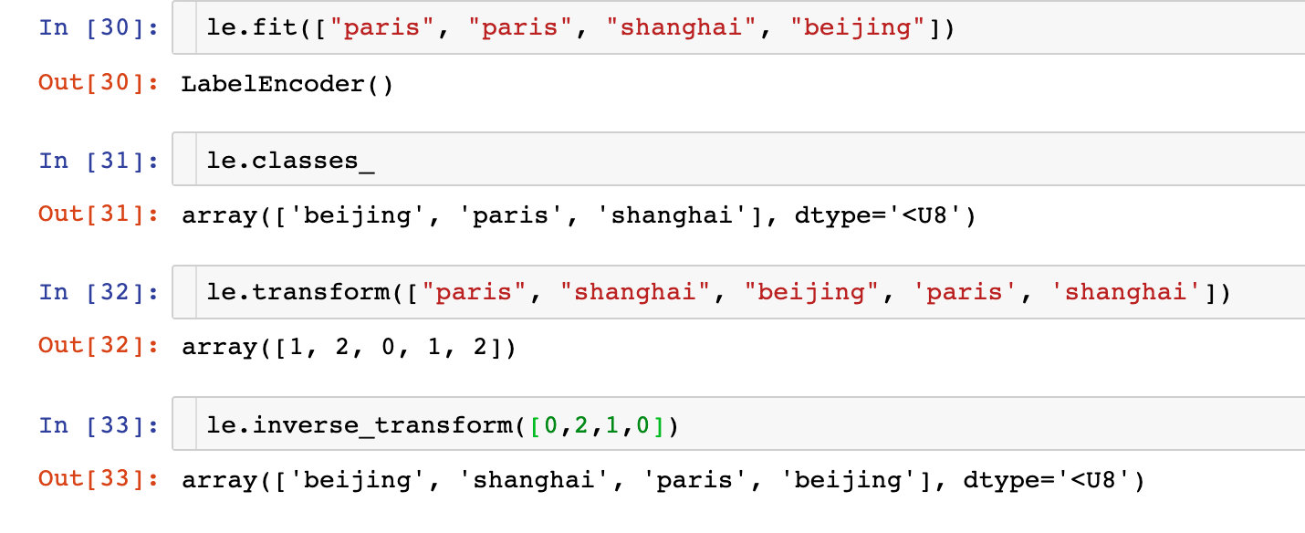
Type code

Cases from the official website: https://scikit-learn.org/stable/modules/generated/sklearn.preprocessing.LabelEncoder.html

Encode numbers

Encoding strings

Modeling case

Import module

from sklearn.neighbors import KNeighborsClassifier, NeighborhoodComponentsAnalysis  # Model
from sklearn.datasets import load_iris  # Import data
from sklearn.model_selection import train_test_split  # Segmentation data
from sklearn.model_selection import GridSearchCV  # Grid search
from sklearn.pipeline import Pipeline  # Pipeline operation

from sklearn.metrics import accuracy_score  # Score verification

Model instantiation

# Model instantiation
knn = KNeighborsClassifier(n_neighbors=5)

Training model

knn.fit(X_train, y_train)

KNeighborsClassifier()

Test set prediction

y_pred = knn.predict(X_test)
y_pred  # Model based prediction

array([0, 0, 2, 2, 1, 0, 0, 2, 2, 1, 2, 0, 1, 2, 2, 0, 2, 1, 0, 2, 1, 2,
       1, 1, 2, 0, 0, 2, 0, 2])

Score verification

There are two ways to verify the model score:

knn.score(X_test,y_test)

0.9333333333333333

accuracy_score(y_pred,y_test)

0.9333333333333333

Grid search

How to search for parameters

from sklearn.model_selection import GridSearchCV

# Search parameters
knn_paras = {"n_neighbors":[1,3,5,7]}
# Default model
knn_grid = KNeighborsClassifier()

# Instanced objects for grid search
grid_search = GridSearchCV(
	knn_grid, 
	knn_paras, 
	cv=10  # 10 fold cross validation
)
grid_search.fit(X_train, y_train)

GridSearchCV(cv=10, estimator=KNeighborsClassifier(),
             param_grid={'n_neighbors': [1, 3, 5, 7]})

# Best parameter value found by search
grid_search.best_estimator_ 

KNeighborsClassifier(n_neighbors=7)

grid_search.best_params_

{'n_neighbors': 7}

grid_search.best_score_

0.975

Search result based modeling

knn1 = KNeighborsClassifier(n_neighbors=7)

knn1.fit(X_train, y_train)

KNeighborsClassifier(n_neighbors=7)

From the following results, we can see that the modeling effect after grid search is better than that without grid search

y_pred_1 = knn1.predict(X_test)

knn1.score(X_test,y_test)

1.0

accuracy_score(y_pred_1,y_test)

1.0