explain
- This article will not introduce all array functions and will not explain all parameters. For details, please refer to the official documents.
- Parameters with square brackets [] can be omitted.
- The output of each small piece of code is written in the comments below.
1, Array creation
1.1 create an array using existing data
| function | effect |
|---|---|
| np.array(object, dtype=None, copy=True) | Objects can be scalars, lists, tuples and other objects. dtype is a data type. Copy controls whether to copy objects; Convert object to n-dimensional array |
| np.asarray(object, dtype=None) | And NP Array () has similar functions. See section 1.1.2 for the differences |
| np.fromfunction(f, shape, dtype=float) | Shape is an integer tuple of size N, and f is a scalar function with N parameters; Returns an array of shape shapes, where each element is the value obtained by passing in f according to its index |
| np.fromstring(s, dtype=float, sep) | s is a string and sep is a separator; Converts a string into an array after it is separated by delimiters |
1.1.1 np.array()
np.array() is the most commonly used method.
""" example 1 """
A = np.array([1, 2])
print(A)
print(type(A))
# [1 2]
# <class 'numpy.ndarray'>

""" example 2 """
A = np.array([(1, 2), (3, 4)])
print(A)
print(type(A))
# [[1 2]
#  [3 4]]
# <class 'numpy.ndarray'>

""" example 3 """
A = np.array([1, 2, 3], dtype=np.complex128)
print(A)
# [1.+0.j 2.+0.j 3.+0.j]

""" example 4 """
A = np.array([1, 2, 3])
B = np.array(A)
print(B)
print(type(B))
# [1 2 3]
# <class 'numpy.ndarray'>

""" example 5 """
A = np.array([1, 2, 3])
B = np.array(A)
C = np.array(A, copy=False)
A[0] = 2
print(B, '\n', C)
# [1 2 3]
# [2 2 3]
It is not difficult to find from example 4 that our object can also be ndarray.
As can be seen from example 5, if copy is turned off, modifying the value of A will affect C (because C points to A at this time). In fact, if A is not ndarray (such as list), no matter what copy is set to, our NP Array () will copy A.
1.1.2 np.asarray()
np.array() and NP Asarray () can convert the source data object into ndarray, but the main difference is that when the source data is ndarray, the array will still copy a copy and occupy new memory, but asarray will not.
The difference can be seen from the following two examples:
""" example 1 """
A = [1, 2, 3]
B = np.array(A)
C = np.asarray(B)
A[0] = 2
print(A, '\n', B, '\n', C, sep='')
# [2, 2, 3]
# [1 2 3]
# [1 2 3]

""" example 2 """
A = np.array([1, 2, 3])
B = np.array(A)
C = np.asarray(A)
A[0] = 2
print(A, '\n', B, '\n', C, sep='')
# [2 2 3]
# [1 2 3]
# [2 2 3]
In order to facilitate memory, we can understand it as follows:
# Loosely speaking, the following two statements are equivalent:
np.array(object, copy=False)
np.asarray(object)
If there is no special need, try to use NP Array () instead of NP asarray().
1.1.3 np.fromfunction()
We first define a function
def f(x, y):
    return x + y
Because f has two parameters, the size of shape should also be 2. We might as well set shape=(3, 2), then the final returned size is 3 × 2 3\times 2 three × Array of 2 Record the array as A A A. So naturally
A [ i ] [ j ] = f ( i , j ) = i + j A[i][j]=f(i,j)=i+j A[i][j]=f(i,j)=i+j
Let's look at the effect:
A = np.fromfunction(f, (3, 2), dtype=int)
print(A)
# [[0 1]
#  [1 2]
#  [2 3]]
If we use python's anonymous function, we only need one line of code:
A = np.fromfunction(lambda x, y: x + y, (3, 2), dtype=int)
Use NP Fromfunction(), we can easily create an array whose elements are related to the index. For example, for the following arrays:
[ T r u e F a l s e F a l s e F a l s e T r u e F a l s e F a l s e F a l s e T r u e ] \begin{bmatrix} \mathrm{True} & \mathrm{False} & \mathrm{False} \\ \mathrm{False} & \mathrm{True} & \mathrm{False} \\ \mathrm{False} & \mathrm{False} & \mathrm{True} \\ \end{bmatrix} ⎣⎡TrueFalseFalseFalseTrueFalseFalseFalseTrue⎦⎤
We can create it this way:
A = np.fromfunction(lambda i, j: i == j, (3, 3))
1.1.4 np.fromstring()
For the following string:
s = '1 2 3 4 5'
To convert it to an integer array, our first reaction is:
A = np.array(list(map(int, s.split())))
print(A)
# [1 2 3 4 5]
But use NP Fromstring(), we can complete the creation more conveniently. Note that each number in the string is separated by spaces, so you only need to set sep = '':
A = np.fromstring(s, dtype=int, sep=' ')
print(A)
# [1 2 3 4 5]
1.2 create an array based on the range of values
| function | effect |
|---|---|
| np.arange([start], stop, [step], dtype=None) | Create an array within the [start, stop) interval with step size; if start is omitted, it defaults to 0 and if step is omitted, it defaults to 1 |
| np.linspace(start, stop, num=50, endpoint=True, dtype=None) | Create an array with the size of num in the [start, stop] interval; When the endpoint is closed, the interval becomes [start, stop] |
| np.logspace(start, stop, num=50, endpoint=True, base=10.0, dtype=None) | Equivalent to NP Based on the result of linspace (), for each element a a a make transformation a : = b a s e a a:=base^a a:=basea |
| np.geomspace(start, stop, num=50, endpoint=True, dtype=None) | And NP Logspace () is similar, except NP Geomspace () automatically selects the appropriate substrate |
1.2.1 np.arange()
""" example 1 """
A = np.arange(6)
B = np.arange(2, 6)
C = np.arange(2, 10, 2)
print(A, '\n', B, '\n', C, sep='')
# [0 1 2 3 4 5]
# [2 3 4 5]
# [2 4 6 8]

""" example 2 """
A = np.arange(6, -1, -1, dtype=float)
print(A)
# [6. 5. 4. 3. 2. 1. 0.]

""" example 3 """
A = np.arange(6, -1, -1.0)
print(A)
# [6. 5. 4. 3. 2. 1. 0.]
Note: when the value of start is much larger than the value of step, NP The expected result may not be returned by orange (), so NP. Is needed Linspace()
1.2.2 np.linspace()
np.linspace() returns a float ing-point array by default
""" example 1 """
A = np.linspace(1, 10, 10)
B = np.linspace(1, 10, 10, endpoint=False)
print(A, '\n', B, sep='')
# [ 1.  2.  3.  4.  5.  6.  7.  8.  9. 10.]
# [1.  1.9 2.8 3.7 4.6 5.5 6.4 7.3 8.2 9.1]
1.2.3 np.logspace()
This function is similar to NP Linspace () function is closely related. Let's first look at NP An example of linspace():
A = np.linspace(1, 5, 5)
print(A)
# [1. 2. 3. 4. 5.]
Replace linspace with logspace and set the base to 2:
A = np.logspace(1, 5, 5, base=2)
According to the description in the previous table, the result should be:
[ 2 1 , 2 2 , 2 3 , 2 4 , 2 5 ] [2^1,2^2,2^3,2^4,2^5] [21,22,23,24,25]
The same is true for the output:
# [ 2. 4. 8. 16. 32.]
1.2.4 np.geomspace()
np.logspace() and NP Geomspace() will generate an array with exponential growth. The difference is that the array generated by logspace is:
[ b a s e s t a r t , ⋯ , b a s e s t o p ] [base^{start},\cdots,base^{stop}] [basestart,⋯,basestop]
The array generated by geomspace is:
[ s t a r t , ⋯ , s t o p ] [start,\cdots,stop] [start,⋯,stop]
For example, if you set start=1, stop=1000, num=4, geomspace will automatically select base 10:
A = np.geomspace(1, 1000, num=4, dtype=int)
print(A)
# [   1   10  100 1000]
1.3 creating arrays of specific types
| function | effect |
|---|---|
| np.empty(shape) | List of integers / shapes; Returns an empty array of shape shapes (uninitialized array) |
| np.empty_like(prototype) | prototype is a given array; Returns an empty array with the same shape as the given array |
| np.ones(shape) | Returns a full 1 array of shape shapes |
| np.ones_like(prototype) | Returns an all 1 array with the same shape as the given array |
| np.zeros(shape) | Returns an all 0 array of shape shapes |
| np.zeros_like(prototype) | Returns an all 0 array with the same shape as the given array |
| np.full(shape, value) | Value is scalar or array; When value is a scalar, it returns a full value array with the same shape as the shape; See section 1.3.4 for the case where value is an array |
| np.full_like(prototype, value) | Returns a full value array with the same shape as the given array |
| np.eye(m, n=m, k=0) | m is the number of rows of the matrix, n is the number of columns of the matrix, and k controls the diagonal; Returns a matrix (array) whose main diagonal is all 1 and other positions are all 0 |
| np.identity(n) | Returns the identity matrix of order n |
1.3.1 np.empty()
Unlike zeros, empty does not initialize elements to 0 (but it does not mean there are no numbers in the array), so it may be faster than zeros.
""" example 1 """
A = np.empty(2)
print(A)
# [4.64929150e+143 2.37662553e-045]

""" example 2 """
A = np.empty([2, 2])
print(A)
# [[ 1.05328699e-311 -6.77097176e-233]
#  [ 1.05328694e-311  1.05328694e-311]]

""" example 3 """
A = np.array([1, 2, 3])
B = np.empty_like(A)
print(B)
# [5111887 5701703 5111877]
1.3.2 np.ones()
""" example 1 """
A = np.ones([2, 2])
print(A)
# [[1. 1.]
#  [1. 1.]]

""" example 2 """
A = np.array([1, 2, 3])
B = np.ones_like(A)
print(B)
# [1 1 1]
1.3.3 np.zeros()
""" example 1 """
A = np.zeros(5)
print(A)
# [0. 0. 0. 0. 0.]

""" example 2 """
A = np.array([1, 2, 3])
B = np.zeros_like(A)
print(B)
# [0 0 0]
1.3.4 np.full()
""" example 1 """
A = np.full((2, 3), 3)
print(A)
# [[3 3 3]
#  [3 3 3]]

""" example 2 """
A = np.full((3, 3), [1, 2, 3])
print(A)
# [[1 2 3]
#  [1 2 3]
#  [1 2 3]]
It can be seen that when value is an array, each row in the returned array is filled with value. It should be noted that in this case, shape[1] should be consistent with len(value), otherwise an error will be reported:
A = np.full((3, 4), [1, 2, 3])
print(A)
# ValueError: could not broadcast input array from shape (3,) into shape (3,4)
Let's look at NP full_ like():
A = np.arange(6, dtype=int)
B = np.full_like(A, 1)
C = np.full_like(A, 0.1)
D = np.full_like(A, 0.1, dtype=float)
print(A, '\n', B, '\n', C, '\n', D, sep='')
# [0 1 2 3 4 5]
# [1 1 1 1 1 1]
# [0 0 0 0 0 0]
# [0.1 0.1 0.1 0.1 0.1 0.1]
1.3.5 np.eye()
Let's introduce the diagonal first.
Main diagonal:
( 0 , 0 ) → ( 1 , 1 ) → ⋯ → ( s , s ) (0,0)\to(1,1)\to\cdots\to(s,s) (0,0)→(1,1)→⋯→(s,s)
For example, in the following two matrices, the path of 1 is the main diagonal:
[ 1 0 0 1 ] , [ 1 0 0 0 1 0 ] \begin{bmatrix} 1 & 0 \\ 0 & 1 \\ \end{bmatrix},\quad \begin{bmatrix} 1 & 0 & 0\\ 0 & 1 & 0\\ \end{bmatrix} [1001],[100100]
Sub diagonal:
T y p e I : ( 0 , 0 + k ) → ( 1 , 1 + k ) → ⋯ → ( s , s + k ) , k ≥ 1 T y p e I I : ( 0 − k , 0 ) → ( 1 − k , 1 ) → ⋯ → ( s − k , s ) , k ≤ − 1 \mathrm{Type \;I}:\; (0,0+k)\to(1,1+k)\to\cdots\to(s,s+k),\quad k\geq 1 \\ \mathrm{Type \;II}:\; (0-k,0)\to(1-k,1)\to\cdots\to(s-k,s),\quad k\leq -1 \\ TypeI:(0,0+k)→(1,1+k)→⋯→(s,s+k),k≥1TypeII:(0−k,0)→(1−k,1)→⋯→(s−k,s),k≤−1
among k k k is an integer
Let's first look at the first type of sub diagonal, and we might as well set it k = 1 k=1 k=1, then the path is
( 0 , 1 ) → ( 1 , 2 ) → ( 2 , 3 ) → ⋯ → ( s , s + 1 ) (0,1)\to(1,2)\to(2,3)\to\cdots\to(s,s+1) (0,1)→(1,2)→(2,3)→⋯→(s,s+1)
For example, in the following two matrices, the path of 1 is the first type sub diagonal:
[ 0 1 0 0 0 1 0 0 0 ] , [ 0 1 0 0 0 0 0 1 0 0 0 0 0 1 0 ] \begin{bmatrix} 0 & 1 & 0\\ 0 & 0 & 1\\ 0 & 0 & 0\\ \end{bmatrix},\quad \begin{bmatrix} 0 & 1 & 0&0&0\\ 0 & 0 & 1&0&0\\ 0 & 0 & 0&1&0\\ \end{bmatrix} ⎣⎡000100010⎦⎤,⎣⎡000100010001000⎦⎤
It is equivalent to the upward translation of the main diagonal k k k units to get the first type of sub diagonal.
If you look at the second type of diagonal, you might as well set it k = − 1 k=-1 k = − 1, then the path is:
( 1 , 0 ) → ( 2 , 1 ) → ( 3 , 2 ) → ⋯ → ( s + 1 , s ) (1,0)\to(2,1)\to(3,2)\to\cdots\to(s+1,s) (1,0)→(2,1)→(3,2)→⋯→(s+1,s)
For example, in the following two matrices, the path of 1 is the second type sub diagonal:
[ 0 0 0 1 0 0 0 1 0 ] , [ 0 0 0 1 0 0 0 1 0 0 0 1 0 0 0 ] \begin{bmatrix} 0 & 0 & 0\\ 1 & 0 & 0\\ 0 & 1 & 0\\ \end{bmatrix},\quad \begin{bmatrix} 0 & 0 & 0\\ 1 & 0 & 0\\ 0 & 1 & 0\\ 0 & 0 & 1 \\ 0 & 0 & 0 \\ \end{bmatrix} ⎣⎡010001000⎦⎤,⎣⎢⎢⎢⎢⎡010000010000010⎦⎥⎥⎥⎥⎤
It is equivalent to the downward translation of the main diagonal − k -k − k units to get the second type of sub diagonal.
So we can make a summary:
- k = 0 k=0 When k=0, it is the main diagonal.
- k > 0 k>0 k> 0 is the first type of sub diagonal, which is equivalent to the upward translation of the main diagonal k k k units.
- k < 0 k<0 When k < 0, it is the second type of sub diagonal, which is equivalent to the downward translation of the main diagonal − k -k − k units.
For the sake of convenience, we use "the third party" uniformly k k All diagonals are called "k diagonals". For example, section 0 0 0 diagonal is the main diagonal, the second diagonal 1 1 1 diagonal is obtained by translating the main diagonal upward by 1 unit, and the second diagonal is obtained − 1 -1 − 1 diagonal is obtained by translating the main diagonal downward by 1 unit.
After knowing what diagonal is, the following example is not difficult to understand:
""" example 1 """
A = np.eye(3)
print(A)
# [[1. 0. 0.]
#  [0. 1. 0.]
#  [0. 0. 1.]]

""" example 2 """
A = np.eye(3, 5)
print(A)
# [[1. 0. 0. 0. 0.]
#  [0. 1. 0. 0. 0.]
#  [0. 0. 1. 0. 0.]]

""" example 3 """
A = np.eye(3, 4, k=2)
print(A)
# [[0. 0. 1. 0.]
#  [0. 0. 0. 1.]
#  [0. 0. 0. 0.]]

""" example 4 """
A = np.eye(5, 3, k=-3)
print(A)
# [[0. 0. 0.]
#  [0. 0. 0.]
#  [0. 0. 0.]
#  [1. 0. 0.]
#  [0. 1. 0.]]
1.3.6 np.identity()
The following three statements are equivalent:
np.eye(n)
np.eye(n, n)
np.identity(n)
1.4 create diagonal matrix and upper / lower triangular matrix
| function | effect |
|---|---|
| np.diag(v, k=0) | K control diagonal; When v is a two-dimensional array, the k-th diagonal is returned as a one-dimensional array; When v is a one-dimensional array, the array will be taken as the k-th diagonal and the diagonal matrix will be constructed |
| np.tri(m, n=m, k=0) | Create an m × The matrix of n, in which the k diagonal and its following parts are all 1, and the other positions are all 0 |
| np.tril(object, k=0) | Object is a two-dimensional array; Returns a copy of an object, where the part above the k diagonal of the copy is set to 0 |
| np.triu(object, k=0) | Returns a copy of an object, where the part below the k diagonal of the copy is set to 0 |
1.4.1 np.diag()
""" example 1 """
A = np.array([[1, 2], [3, 4]])
print(np.diag(A))
print(np.diag(A, k=1))
# [1 4]
# [2]

""" example 2 """
A = np.array([1, 2, 3])
print(np.diag(A))
print(np.diag(A, k=1))
# [[1 0 0]
#  [0 2 0]
#  [0 0 3]]
# [[0 1 0 0]
#  [0 0 2 0]
#  [0 0 0 3]
#  [0 0 0 0]]
1.4.2 np.tri()
""" example 1 """
A = np.tri(3, 4, k=1)
print(A)
# [[1. 1. 0. 0.]
#  [1. 1. 1. 0.]
#  [1. 1. 1. 1.]]

""" example 2 """
A = np.tri(3, 4, k=-1)
print(A)
# [[0. 0. 0. 0.]
#  [1. 0. 0. 0.]
#  [1. 1. 0. 0.]]

""" example 3 """
A = np.tri(2, k=-1)
print(A)
# [[0. 0.]
#  [1. 0.]]
1.4.3 np.tril()
""" example 1 """
A = np.array([[1, 2, 3], [4, 5, 6], [7, 8, 9]])
print(np.tril(A))
# [[1 0 0]
#  [4 5 0]
#  [7 8 9]]

""" example 2 """
A = np.array([[1, 2, 3], [4, 5, 6], [7, 8, 9]])
print(np.tril(A, k=-1))
# [[0 0 0]
#  [4 0 0]
#  [7 8 0]]
1.4.4 np.triu()
""" example 1 """
A = np.array([[1, 2, 3], [4, 5, 6], [7, 8, 9]])
print(np.triu(A))
# [[1 2 3]
#  [0 5 6]
#  [0 0 9]]

""" example 2 """
A = np.array([[1, 2, 3], [4, 5, 6], [7, 8, 9]])
print(np.triu(A, k=1))
# [[0 2 3]
#  [0 0 6]
#  [0 0 0]]
2, Basic operation of array
2.1 viewing array information
We already know that in Numpy, one-dimensional arrays represent vectors and two-dimensional arrays represent matrices. For three-dimensional and above arrays, we need to call them tensors.
In Numpy, the dimension of the array has another name - axes, and a few dimensional array has several axes. For example, for the following two-dimensional array:
[[0., 0., 0.],
 [1., 1., 1.]]
It has two axes, and the length of the array along the first axis is 2 and the length along the second axis is 3, that is:
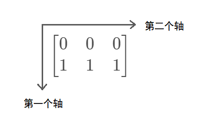
Seeing this, you may wonder why the first axis is along the row direction and the second axis is along the column direction? Why not have the first axis in the column direction and the second axis in the row direction?
This is because when we index, the index form is as follows: A [ i ] [ j ] A[i][j] A[i][j]. The row index is in the first position and the column index is in the second position, so our first axis is specified as along the row direction and the second axis is specified as along the column direction.
For an N-dimensional array, we also call N the rank of the array.
We have the following methods to view the information of the array:
| method | effect |
|---|---|
| ndarray.ndim | Returns the dimension (rank) of the array |
| ndarray.shape | Returns the shape of the array in tuple form; For example, for a two-dimensional array, the returned form is (m, n) |
| ndarray.size | Returns the total number of elements in the array; This is equal to the product of all elements in the shape |
| ndarray.dtype | Returns the data type of the array (because the array requires that the data types of all elements in it must be the same) |
Let's learn more about these methods through an example:
A = np.array([[1, 2, 3], [4, 5, 6]])
print(A.ndim)
print(A.shape)
print(A.size)
print(A.dtype)
# 2
# (2, 3)
# 6
# int32
2.2 arithmetic operators
Applying arithmetic operators to an array will be processed by element (also known as element by element).
A = np.array([1, 2, 3])
B = np.array([4, 5, 6])

print(A + B)
# [5 7 9]
print(B - A)
# [3 3 3]
print(A + 2)
# [3 4 5]
print(A * 2)
# [2 4 6]
print(A / 2)
# [0.5 1.  1.5]
print(A ** 2)
# [1 4 9]
print(A * B)
# [ 4 10 18]
print(A ** B)
# [  1  32 729]
print(A >= 2)
# [False  True  True]
When an array with different precision (data type) is operated, the precision (data type) of the result is the highest precision (up conversion) of the array involved in the operation.
For example, adding two arrays with data types of int32 and float64 will result in an array with precision of float64:
A = np.array([1, 2, 3], dtype=int)
B = np.array([4, 5, 6], dtype=float)
C = A + B
print(C)
print(C.dtype)
# [5. 7. 9.]
# float64
Add two arrays with data types of float64 and complex128 respectively, and the result will be an array with precision of complex128:
A = np.array([1, 2, 3], dtype=complex)
B = np.array([4, 5, 6], dtype=float)
C = A + B
print(C)
print(C.dtype)
# [5.+0.j 7.+0.j 9.+0.j]
# complex128
2.3 indexing and slicing
Numpy's n-dimensional array can be indexed, assigned, sliced, iterated and other operations like Python's list.
2.3.1 indexing
The index and assignment methods of n-dimensional array are the same as those of the list:
A = np.arange(12)
print(A[3])
# 3
A[5] = 9
print(A)
# [ 0  1  2  3  4  9  6  7  8  9 10 11]
Of course, we can also index multiple elements at the same time:
A = np.arange(12)
indexes_1 = np.array([1, 4, 7, 9])
indexes_2 = [1, 4, 7, 9]
print(A[indexes_1])
print(A[indexes_2])
# [1 4 7 9]
# [1 4 7 9]
It can be seen that when indexes is an n-dimensional array or list, the index of multiple elements can be completed, but when indexes is a tuple, the index will fail.
For a two-dimensional list, the method of indexing an element is A [ i ] [ j ] A[i][j] A[i][j]. However, in two-dimensional arrays, there is another method besides this method: A [ i , j ] A[i, j] A[i,j].
A = np.array([[1, 2, 3], [4, 5, 6]])
print(A[0, 1])
print(A[1, -1])
# 2
# 6
Please use A [ i , j ] A[i, j] A[i,j], its efficiency ratio A [ i ] [ j ] A[i][j] A[i][j] higher.
If the index number is less than the dimension of the array, a sub array is obtained:
A = np.array([[1, 2, 3], [4, 5, 6]])
print(A[0]) # It is equivalent to taking line 0 of A
# [1 2 3]
Back to the one-dimensional array, if the array capacity is very large and we need to index many elements, is there a simpler method?
The answer is slicing.
2.3.2 slicing
- Not only n-dimensional arrays and lists, any ordered sequence in python supports slicing, such as strings, tuples, etc.
- The result type returned by slicing is consistent with the type of sliced object. Slice the array to get the array, slice the list to get the list, and slice the string to get the string.
Next, we will only discuss array slicing. Its standard format is:
A [ s t a r t : s t o p : s t e p ] , s t e p ≠ 0 A[start:stop:step],\quad step\neq0 A[start:stop:step],step=0
Start is the slice start index and end is the slice end index. Note that here is the left open right closed interval, i.e [ s t a r t , s t o p ) [start, stop) [start,stop).
When step is omitted, it defaults to 1, and the symbol of step determines the direction of slice: when step is positive, forward slice is executed; When step is negative, reverse slicing is performed.
For example:
A = np.arange(10)
print(A[1:6:1])
print(A[5:0:-1])
# [1 2 3 4 5]
# [5 4 3 2 1]
Suppose step gives:
- If only stop is omitted, it will slice along the slice direction from start to an end point of the array (including the end point).
- If only start is omitted, it will slice from one end of the array along the slice direction to stop (excluding stop).
For example:
A = np.arange(10)
print(A[1::1])
print(A[:0:-1])
# [1 2 3 4 5 6 7 8 9]
# [9 8 7 6 5 4 3 2 1]
- If both start and stop are omitted, the array will be sliced from one end point to the other end point (including the end point) along the slicing direction
For example:
A = np.arange(10)
print(A[::1])
print(A[::-1])
# [0 1 2 3 4 5 6 7 8 9]
# [9 8 7 6 5 4 3 2 1 0]
So we got a method to quickly reverse the array:
A = A[::-1]
Because when step is 1, it can be omitted, and a colon can be further omitted, that is, the following three statements are equivalent:
A[start:stop:1]
A[start:stop:]
A[start:stop]
So we can also get a method to copy the array:
B = A[:]
After being familiar with slicing, we can complete more complex operations, such as the following matrix:
A = [ 1 2 3 4 5 6 7 8 9 10 11 12 13 14 15 16 ] A= \begin{bmatrix} 1 & 2 & 3 & 4 \\ 5 & 6 & 7 & 8 \\ 9 & 10 & 11 & 12 \\ 13 & 14 & 15 & 16 \\ \end{bmatrix} A=⎣⎢⎢⎡15913261014371115481216⎦⎥⎥⎤
If we want to take it out A A In the last three lines of A, you can do this:
# The following two statements are equivalent. Try to think about why they are equivalent
print(A[1:, :])
print(A[1:])
If we want to take it out A A The last three columns of A should do this:
# Try to think about why there is only one solution
print(A[:, 1:])
To get 2 , 4 , 10 , 12 2, 4, 10, 12 For the four elements 2, 4, 10 and 12, we only need to index (slice) as follows:
# It is equivalent to taking the elements at the intersection of row 0 and row 3 with column 1 and column 3
print(A[::2, 1::2])
# [[ 2  4]
#  [10 12]]
2.3.3 advanced index
In this section, we will discuss more advanced indexing (slicing), which can help you select certain elements easily and quickly.
2.3.3.1 use of ellipsis (...)
Returning to section 2.3.1, we know that for a two-dimensional array, take out the first sub array along the first axis (i.e. take row 0), you should use A[0]. In fact, it is equivalent to A[0,:]. For a three-dimensional array, take its k-th sub array in the third axis direction. We should use a [:,:, k]. At this time, we don't have a more concise representation.
So the problem comes. For N-dimensional arrays, when N is very large, if we want to get its k-th sub array on a certain axis, our index will involve a large number of colons and commas, and manual input is unrealistic. How to solve this problem?
Fortunately, Numpy provides a more concise representation. When there are two or more colons, we can use three points Instead. For example, for the second example above, we can simply write A[..., k].
If A is A five-dimensional array, then:
- A[1,2,...] Equivalent to a [1,2,:,:,:]
- A[...,3] is equivalent to A[:,:,:,:,3]
- A[4,...,5,:] is equivalent to A[4,:,:,5,:]
ellipsis... Occurs at most once in the index.
Let's take an example of a three-dimensional array:
A = np.array([[[0, 1, 2],
			   [10, 12, 13]],
			  [[100, 101, 102],
			   [110, 112, 113]]])
print(A[1, :, :])
print(A[1, ...])
# [[100 101 102]
#  [110 112 113]]
# [[100 101 102]
#  [110 112 113]]

print(A[..., 2])
# [[  2  13]
#  [102 113]]
2.3.3.2 index with index array
In section 2.3.1, we mentioned that n-dimensional arrays or lists can be used to index multiple elements. In order to be closer to Numpy, next, we abandon the list and use only n-dimensional arrays to index. This method is also called using index array for indexing.
Let's start with a simple example:
A = np.arange(12)
i = np.array([0, 1, 4, 7])
print(A[i])
# [0 1 4 7]
When our index array is a two-dimensional array, the returned result is also a two-dimensional array:
A = np.arange(12)
i = np.array([[0, 1], [4, 7]])
print(A[i])
# [[0 1]
#  [4 7]]
We can mathematically extend it to a more general form, assuming that indexes is k k k-dimensional array, i.e.:
i n d e x e s [ i 1 , i 2 , ⋯ , i k ] = a i 1 i 2 ⋯ i k indexes[i_1,i_2,\cdots,i_k]=a_{i_1i_2\cdots i_k} indexes[i1,i2,⋯,ik]=ai1i2⋯ik
Thus, the indexed result A[indexes] meets:
A [ i n d e x e s ] [ i 1 , i 2 , ⋯ , i k ] = A [ a i 1 i 2 ⋯ i k ] A[indexes][i_1,i_2,\cdots,i_k]=A[a_{i_1i_2\cdots i_k}] A[indexes][i1,i2,⋯,ik]=A[ai1i2⋯ik]
We can also provide indexes for multiple dimensions, but note that the index array of each dimension must have the same shape:
A = np.array([[0, 1, 2, 3],
			  [4, 5, 6, 7],
			  [8, 9, 10, 11]])

i = np.array([[0, 1],
			  [1, 2]])
j = np.array([[2, 1],
			  [3, 3]])

print(A[i, j])
# [[ 2  5]
#  [ 7 11]]

print(A[i, 2])
# [[ 2  6]
#  [ 6 10]]

print(A[i, :])
# [[[ 0  1  2  3]
#   [ 4  5  6  7]]
#  [[ 4  5  6  7]
#   [ 8  9 10 11]]]
Since we can index multiple elements, we should also be able to assign values to multiple elements:
""" example 1 """
A = np.array([0, 1, 2, 3, 4])
A[[0, 1, 3]] = 5
print(A)
# [5 5 2 5 4]

""" example 2 """
A = np.array([0, 1, 2, 3, 4])
A[[0, 1, 3]] = [7, 8, 9]
print(A)
# [7 8 2 9 4]

""" example 3 """
A = np.array([0, 1, 2, 3, 4])
A[[0, 1, 3]] = A[[0, 1, 3]] + 1
print(A)
# [1 2 2 4 4]

""" example 4 """
A = np.array([0, 1, 2, 3, 4])
A[[0, 0, 3]] += 1
print(A)
# [1 1 2 4 4]
As you can see, in example 4, 0 0 The value of 0 has only increased once. Why?
This is because A[[0, 0, 3]] itself is [0, 0, 3]. Executing A[[0, 0, 3]] += 1 is equivalent to executing A[[0, 0, 3]] = A[[0, 0, 3]] + 1, which is equivalent to executing A[[0, 0, 3]] = [1,1,4]. This statement is equivalent to
A[0] = 1
A[0] = 1
A[3] = 4
It can be seen that A[0] is assigned repeatedly, so its value will not increase twice.
What if we want to increase the value of A[0] twice (on the basis of keeping A[3] only increased once)?
We only need to modify the assignment:
A[[0, 0, 3]] += [x, 2, 1]
Where x can be any number, because then the value of A[0] will be overwritten by 2. The above statement is equivalent to:
A[0] = x
A[0] = 2
A[3] = 1
2.3.3.3 index with Boolean array
Let's start with an example:
A = np.array([[1, 2, 3],
			  [4, 5, 6]])
i = np.array([[True, False, False],
			  [False, False, True]])
print(A[i])
# [1 6]
It can be seen that we only index the places where it is True, while the places where it is False are not indexed.
Using this feature, we can complete some interesting operations. For example, for the above array A, if you want the elements greater than or equal to 3 in A to be set to 0, we can first create A Boolean array and then assign A value:
A = np.array([[1, 2, 3], [4, 5, 6]])
i = A >= 3
print(i)
# [[False False  True]
#  [ True  True  True]]

A[i] = 0
print(A)
# [[1 2 0]
#  [0 0 0]]
Let's look at a few more examples to further familiarize ourselves with Boolean array indexes:
A = np.array([[1, 2, 3],
		      [5, 6, 7]])
i = np.array([False, True])
j = np.array([True, False, True])

print(A[i, :])
# [[5 6 7]]

print(A[:, j])
# [[1 3]
#  [5 7]]

print(A[i, j])
# [5 7]
2.4 broadcasting
Numpy uses a broadcast mechanism when dealing with two or more arrays of different shapes. In short, it is to expand one of the arrays or expand two arrays at the same time so that their shapes are the same, so as to continue the operation.
2.4.1 scalar and one-dimensional array
For example, in the operation of scalar * array, the broadcast mechanism is adopted:
a = np.array([1, 2, 3])
b = 2
print(a * b)
# [2 4 6]
When calculating A * b, Numpy will expand b into an array of the same size as A, and then perform the operation by element (the arithmetic operator is operated by element, and the operation by element requires the same shape of the two arrays):
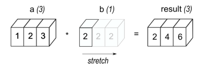
When a large (shape) array and a small (shape) array are operated on, the small array will expand into an array with the same shape as the large array by copying itself. This process is called broadcasting. As we'll see later, not all arrays can be broadcast.
For the above example, we can also do this:
a = np.array([1, 2, 3])
b = np.array([2, 2, 2])
print(a * b)
Their results are the same, but it is undoubtedly better to use the broadcast mechanism, because the broadcast mechanism occupies less memory space and is more convenient to use.
2.4.2 one dimensional array and two-dimensional array
Consider the case of one-dimensional array + two-dimensional array. Because + is an arithmetic operator, it needs to operate according to elements, but their shapes are different. Therefore, Numpy will adopt the broadcast mechanism: one-dimensional array expands into an array with the same shape as two-dimensional array by copying itself.
a = np.array([[0, 0, 0],
			  [10, 10, 10],
			  [20, 20, 20],
			  [30, 30, 30]])
b = np.array([1, 2, 3])
print(a + b)
# [[ 1  2  3]
#  [11 12 13]
#  [21 22 23]
#  [31 32 33]]
The specific broadcasting process is as follows:
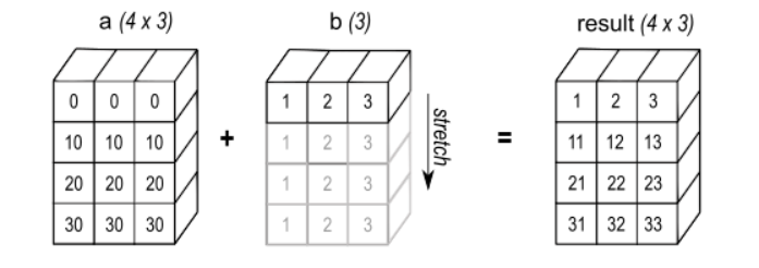
b here is a row vector, so it will broadcast along the row direction (i.e. downward); If b is a column vector, it will broadcast along the column direction (i.e. to the right).
a = np.array([[0, 0, 0],
			  [10, 10, 10],
			  [20, 20, 20],
			  [30, 30, 30]])
b = np.array([[1],
			  [2],
			  [3],
			  [4]])
print(a + b)
# [[ 1  1  1]
#  [12 12 12]
#  [23 23 23]
#  [34 34 34]]
The specific schematic diagram is not given here, please imagine by yourself.
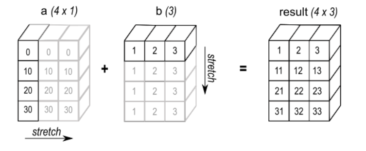
2.4.3 one dimensional array (column vector) and one dimensional array (row vector)
Considering the case of column vector + row vector, Numpy will broadcast two arrays at the same time, expand them into two-dimensional arrays, and then add by element.
a = np.array([[0],
			  [10],
			  [20],
			  [30]])
b = np.array([1, 2, 3])
print(a + b)
# [[ 1  2  3]
#  [11 12 13]
#  [21 22 23]
#  [31 32 33]]
The specific broadcasting process is as follows:
2.4.4 broadcasting rules
Seeing this, readers may wonder when they can broadcast and when they can't broadcast?
Let's define it as follows:
For an N-dimensional array, it has N axes. We can get the shape of the array by using the shape method and present it in tuple form: ( a 1 , a 2 , ⋯ , a N ) (a_1,a_2,\cdots,a_N) (a1, a2,..., aN). For the convenience of narration, we express it as
a 1 × a 2 × ⋯ × a N (A) a_1\times a_2\times\cdots\times a_N\tag{A} a1×a2×⋯×aN(A)
For example, for a 5 5 5 lines 3 3 3-column matrix (two-dimensional array), whose shape is 5 × 3 5\times 3 5×3.
Now consider an M-dimensional array (where M < N M<N M < n), whose shape is
b 1 × b 2 × ⋯ × b M b_1\times b_2\times\cdots\times b_M b1×b2×⋯×bM
In order to ensure the consistency of subscripts after right alignment, we assume that the shape of M-dimensional array is
b k × ⋯ × b N (B) b_k\times\cdots\times b_{N}\tag{B} bk×⋯×bN(B)
And shall meet N − k + 1 = M N-k+1=M N − k+1=M, i.e k = N − M + 1 ≥ 2 k=N-M+1\geq2 k=N−M+1≥2.
Now we will ( B ) (B) (B) Arranged in ( A ) (A) (A) Below the formula and perform right alignment, there are:
a 1 × a 2 × ⋯ × a k × a k + 1 × ⋯ × a N b k × b k + 1 × ⋯ × b N \begin{aligned} a_1\times a_2\times\cdots\times\,\, &a_k \times a_{k+1}\times\cdots\times a_N \\ &b_k\;\!\times b_{k+1}\;\!\times\cdots\times b_N \\ \end{aligned} a1×a2×⋯×ak×ak+1×⋯×aNbk×bk+1×⋯×bN
Here is another definition: ( a i , b i ) (a_i,b_i) (ai, bi) is called compatible if and only if a i = b i a_i=b_i ai = bi or a i a_i ai # and b i b_i One of bi , is 1 1 1.
So we got the broadcast rules: if ( a i , b i ) , k ≤ i ≤ N (a_i,b_i),\; k\leq i\leq N (ai, bi), k ≤ i ≤ N are compatible, then the M-dimensional array can be broadcast.
Let's consolidate this concept through several examples:
""" Broadcasted """
A      (4d array):  8 x 1 x 6 x 1
B      (3d array):      7 x 1 x 5
Result (4d array):  8 x 7 x 6 x 5

A      (2d array):  5 x 4
B      (1d array):      1
Result (2d array):  5 x 4

A      (2d array):  5 x 4
B      (1d array):      4
Result (2d array):  5 x 4

A      (3d array):  15 x 3 x 5
B      (3d array):  15 x 1 x 5
Result (3d array):  15 x 3 x 5

A      (3d array):  15 x 3 x 5
B      (2d array):       3 x 5
Result (3d array):  15 x 3 x 5

A      (3d array):  15 x 3 x 5
B      (2d array):       3 x 1
Result (3d array):  15 x 3 x 5

""" Non broadcast """
A      (1d array):  3
B      (1d array):  4

A      (2d array):      2 x 1
B      (3d array):  8 x 4 x 3
In case of non broadcasting, the program will report an error: valueerror: operators could not be broadcast together with shapes