Principles

Principle here , we can see from the principle that the K-means algorithm mainly has three parts - random initialization, clustering division and moving aggregation.

Random initialization

Using the randperm function, the 1 ∼ m 1\sim m The sequence of 1 ∼ m is randomly disturbed before taking out K K K as initial gathering points.

function centroids = kMeansInitCentroids(X, K)
%KMEANSINITCENTROIDS This function initializes K centroids that are to be 
%used in K-Means on the dataset X
%   centroids = KMEANSINITCENTROIDS(X, K) returns K initial centroids to be
%   used with the K-Means on the dataset X
%

% You should return this values correctly
centroids = zeros(K, size(X, 2));

% ====================== YOUR CODE HERE ======================
% Instructions: You should set centroids to randomly chosen examples from
%               the dataset X
%

% Initialize the centroids to be random examples

%Randomly reorder the indicies of examples
randidx = randperm(size(X,1));
% Take the first K examples
centroids = X(randidx(1:K),:);

% =============================================================

end

Cluster partition

First assume that all points belong to class 1, and then try to update its category from class 2 to K for each point. Matrix multiplication can be used to calculate the distance. Note that the coordinates of sample points and aggregation points here are row vectors.

function idx = findClosestCentroids(X, centroids)
%FINDCLOSESTCENTROIDS computes the centroid memberships for every example
%   idx = FINDCLOSESTCENTROIDS (X, centroids) returns the closest centroids
%   in idx for a dataset X where each row is a single example. idx = m x 1 
%   vector of centroid assignments (i.e. each entry in range [1..K])
%

% Set K
K = size(centroids, 1);

% You need to return the following variables correctly.
idx = ones(size(X,1), 1);

% ====================== YOUR CODE HERE ======================
% Instructions: Go over every example, find its closest centroid, and store
%               the index inside idx at the appropriate location.
%               Concretely, idx(i) should contain the index of the centroid
%               closest to example i. Hence, it should be a value in the 
%               range 1..K
%
% Note: You can use a for-loop over the examples to compute this.
%

for i=1:size(X,1)
    x=X(i,:);
    for k=2:K
        if ((x-centroids(k,:))*(x-centroids(k,:))')<((x-centroids(idx(i),:))*(x-centroids(idx(i),:))')
            idx(i)=k;
        end
    end
end

% =============================================================

end

Mobile gathering point

Update the coordinates of the aggregation point to the average value of other points in the cluster where it is located, and add up the coordinates of other points and divide them by the number of points.

function centroids = computeCentroids(X, idx, K)
%COMPUTECENTROIDS returns the new centroids by computing the means of the 
%data points assigned to each centroid.
%   centroids = COMPUTECENTROIDS(X, idx, K) returns the new centroids by 
%   computing the means of the data points assigned to each centroid. It is
%   given a dataset X where each row is a single data point, a vector
%   idx of centroid assignments (i.e. each entry in range [1..K]) for each
%   example, and K, the number of centroids. You should return a matrix
%   centroids, where each row of centroids is the mean of the data points
%   assigned to it.
%

% Useful variables
[m n] = size(X);

% You need to return the following variables correctly.
centroids = zeros(K, n);


% ====================== YOUR CODE HERE ======================
% Instructions: Go over every centroid and compute mean of all points that
%               belong to it. Concretely, the row vector centroids(i, :)
%               should contain the mean of the data points assigned to
%               centroid i.
%
% Note: You can use a for-loop over the centroids to compute this.
%

cnt=zeros(K,1);
for i=1:m
    centroids(idx(i),:)=centroids(idx(i),:)+X(i,:);
    cnt(idx(i))=cnt(idx(i))+1;
end
centroids=centroids./cnt;


% =============================================================


end

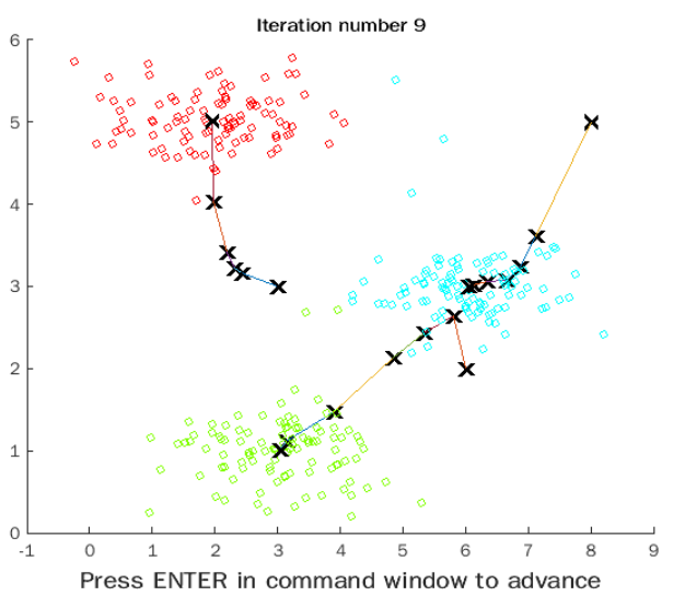
Solving clustering

In order to better show the solution process, there is no random initialization function runkmeans M provided by Wu Enda:

% Load an example dataset
load('ex7data2.mat');
% Settings for running K-Means
max_iters = 10;
For consistency, here we set centroids to specific values but in practice you want to generate them automatically, such as by setting them to be random examples (as can be seen in kMeansInitCentroids).
initial_centroids = [3 3; 6 2; 8 5];

% Run K-Means algorithm. The 'true' at the end tells our function to plot the progress of K-Means
figure('visible','on'); hold on; 
plotProgresskMeans(X, initial_centroids, initial_centroids, idx, K, 1); 
xlabel('Press ENTER in command window to advance','FontWeight','bold','FontSize',14)
[~, ~] = runkMeans(X, initial_centroids, max_iters, true);
set(gcf,'visible','off'); hold off;

function [centroids, idx] = runkMeans(X, initial_centroids, ...
                                      max_iters, plot_progress)
%RUNKMEANS runs the K-Means algorithm on data matrix X, where each row of X
%is a single example
%   [centroids, idx] = RUNKMEANS(X, initial_centroids, max_iters, ...
%   plot_progress) runs the K-Means algorithm on data matrix X, where each 
%   row of X is a single example. It uses initial_centroids used as the
%   initial centroids. max_iters specifies the total number of interactions 
%   of K-Means to execute. plot_progress is a true/false flag that 
%   indicates if the function should also plot its progress as the 
%   learning happens. This is set to false by default. runkMeans returns 
%   centroids, a Kxn matrix of the computed centroids and idx, a m x 1 
%   vector of centroid assignments (i.e. each entry in range [1..K])
%

% Set default value for plot progress
if ~exist('plot_progress', 'var') || isempty(plot_progress)
    plot_progress = false;
end

% Plot the data if we are plotting progress
if plot_progress
    figure;
    hold on;
end

% Initialize values
[m n] = size(X);
K = size(initial_centroids, 1);
centroids = initial_centroids;
previous_centroids = centroids;
idx = zeros(m, 1);

% Run K-Means
for i=1:max_iters
    
    % Output progress
    fprintf('K-Means iteration %d/%d...\n', i, max_iters);
    if exist('OCTAVE_VERSION')
        fflush(stdout);
    end
    
    % For each example in X, assign it to the closest centroid
    idx = findClosestCentroids(X, centroids);
    
    % Optionally, plot progress here
    if plot_progress
        plotProgresskMeans(X, centroids, previous_centroids, idx, K, i);
        previous_centroids = centroids;
        fprintf('Press enter to continue.\n');
        pause;
    end
    
    % Given the memberships, compute new centroids
    centroids = computeCentroids(X, idx, K);
end

% Hold off if we are plotting progress
if plot_progress
    hold off;
end

end

Running in matlab, you can see the continuous movement of aggregation points and the continuous updating of the colors of other points:

Picture compression

A complete picture if its pixels are N × M N\times M N × M. Each pixel is represented in RGB, so one point needs to store three 0 ∼ 255 0\sim 255 0 ∼ 255 unsigned integer, consumption 3 × 8 = 24 3\times 8=24 three × 8 = 24 bytes, the whole picture needs N × M × 24 N\times M\times 24 N × M × 24 bytes. If the color of the picture is compressed, 16 clusters are found, and the average color of each cluster is used to replace the original color, then each pixel only needs to store the color index 1 ∼ 16 1\sim 16 1∼16( 0 ∼ 15 0\sim 15 0 ∼ 15), only 4 4 4 bytes, and then store the divided 16 16 The total space occupied by the color information in 16 is 16 × 24 + N × M × 4 16\times 24+N\times M\times 4 sixteen × 24+N × M × 4. Basically, the picture size can be compressed to the original size 1 6 \frac{1}{6} 61​.

First, use the imread function to read in the picture. At this time, the picture is stored in the N × M × 3 N\times M\times 3 N × M × In the three-dimensional matrix of 3. Then use reshape to convert it into ( N × M ) × 3 (N\times M)\times3 (N × M) × 3, which has become a familiar pattern. Call the K-means algorithm to find the cluster and replace the color of the whole cluster with the color of the aggregation point:

%  Load an image of a bird
A = double(imread('bird_small.png'));
A = A / 255; % Divide by 255 so that all values are in the range 0 - 1

% Size of the image
img_size = size(A);
X = reshape(A, img_size(1) * img_size(2), 3);
K = 16;
max_iters = 10;
initial_centroids = kMeansInitCentroids(X, K);
% Run K-Means
[centroids, ~] = runkMeans(X, initial_centroids, max_iters);
% Find closest cluster members
idx = findClosestCentroids(X, centroids);
X_recovered = centroids(idx,:);

% Reshape the recovered image into proper dimensions
X_recovered = reshape(X_recovered, img_size(1), img_size(2), 3);

% Display the original image 
figure;
subplot(1, 2, 1);
imagesc(A); 
title('Original');
axis square

% Display compressed image side by side
subplot(1, 2, 2);
imagesc(X_recovered)
title(sprintf('Compressed, with %d colors.', K));
axis square

The effect of compression is as follows: