catalogue
Selection mechanism of decision tree
Measurement rules of node purity
Background introduction of decision tree algorithm
Information and quantification of information
Information Gain (used by ID3 algorithm)
Gini index (used by cart algorithm)
Manually adjust the parameters of max depth
min_impurity_decrease parameter
Bring in the best parameters for training
Feature selection of decision tree model
Lightweight and efficient gradient lifting tree feature selection
Bring in the model again for training
Walk into the decision tree
Decision tree is a model widely used in classification and regression tasks. In essence, it learns from layers of if/else problems and draws conclusions.
When it comes to decision tree, the easiest thing to think of is the conditional judgment statement in the program language. if and else is the essence of decision tree.
The following is an analysis of its essence through two cases:
Case 1
Imagine that you want to distinguish between the following four kinds of animals: bears, eagles, penguins and dolphins. Your goal is to get the right answer by asking as few if/else questions as possible. You may first ask: does this animal have feathers? This question will reduce the number of possible animals to only two. If the answer is "yes", you can ask the next question to help you distinguish between eagles and penguins. For example, you can ask if the animal can fly. If the animal has no feathers, it may be a dolphin or a bear, so you need to ask a question to distinguish between the two animals - for example, whether the animal has fins.
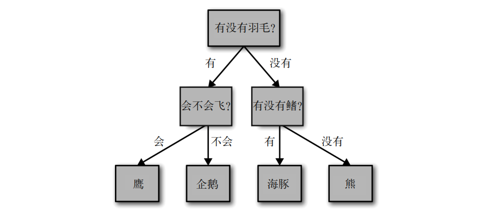
In this diagram, each node of the tree represents a question or an endpoint containing an answer (also known as leaf node). The edge of the tree connects the answer to the next question. In the language of machine learning, in order to distinguish four kinds of animals (eagle, penguin, dolphin and bear), we use three features ("with or without feathers", "can fly" and "with or without fins") to build a model. We can use supervised learning to learn models from data without building models artificially.
Case 2
The ideal is always beautiful, but the reality is really skinny. With the imbalance in the proportion of China's population, many school-age young people will face a severe test, that is, "mate selection", which is the so-called "you look at the scenery on the bridge, and the people who look at the scenery are looking at you". So how many people will consider what factors when looking for the other half? Let's look at a phenomenon diagram of decision tree:
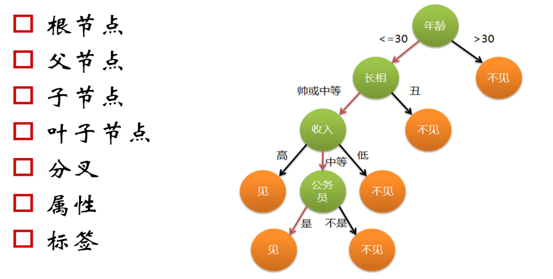
Are you also the above criteria?
Tree of soul
In programming, the judgment conditions that if else depends on are filled in by the programmer, but in machine learning, there are only two things we can do. The first thing is to select the model, the second thing is to put data into the "mouth" of the model, and the rest can only sit aside and worry. The decision tree above depends on us to fill in the discriminant conditions. If it wants to become a real decision tree, it must learn how to select the discriminant conditions. This is the soul of decision tree algorithm, and it is also the key problem to be discussed next.
The first important question is: where do the criteria come from? The data set of classification problem consists of many samples, and each sample data will have multiple feature dimensions. For example, the samples of student data set may contain feature dimensions such as name, age, class and student number. They are also a set, which is called feature dimension set. The feature dimensions of data samples may have some correlation with the final category, and the discriminant conditions of decision tree are generated from this feature dimension set.
Some textbooks believe that only those that really contribute to classification can be called features. These record items in the original data can only be called attributes, while the feature dimension set is called Attribute set. Therefore, in these textbooks, the decision tree selects the discriminant conditions from the set called tree set. Here, in order to maintain the consistency of the language in this book, we still call it "characteristic dimension". Of course, this is just a difference in idioms, and there is no difference in algorithm principle.
Selection mechanism of decision tree
Living experience tells us: pick important questions and ask them first. The decision tree does choose the decision conditions according to this idea. To think about this problem, we can start with "how to be a good decision-making condition". The ultimate goal of decision tree is to solve the classification problem. Of course, the most ideal situation is that after selecting the decision conditions, an if else just divides the data set into two parts according to positive and negative classes.
However, in reality, there is usually no such ideal as "one size fits all". There will always be some samples that are not current affairs "running" into categories that do not belong to them. We retreat to the second place and hope that the fewer impurities in the classification results, the better, that is, the purer the classification results, the better.
According to this goal, the decision tree introduces the concept of "purity". The more samples belonging to the same category in the set, the higher the purity of the set. Every time if else is used for discrimination, the data set of binary classification problem will be divided into two subsets. So how to evaluate the effect of classification? The purity of the subset can be determined. The higher the purity of the subset, the less impurities, and the better the classification effect.
Measurement rules of node purity
There are many classification algorithms using the framework of decision tree, among which the most famous decision tree algorithms are ID3 and C4 5 and CART, the three decision tree algorithms use three different indexes: information gain, gain rate and Gini index as the basis for the selection of decision conditions.
Although the three decision tree algorithms choose three different mathematical indexes, they all have a common purpose: to improve the Purity of nodes under branches.
A large number of binary trees are used in the decision tree algorithm for discrimination. After one discrimination, the most ideal situation is that one branch of the binary tree is purely positive and the other branch is purely negative, which means that a classification is completed completely and accurately. However, most of the discrimination results are not so rational, so a branch will contain both positive and negative classes. However, what we want to see is that the samples contained in a branch belong to the same class as much as possible, that is, the purer the sample category under this branch, the better, so we use "purity" to describe it. There are three things to remember about Purity:
When all samples under a branch belong to the same class, the purity reaches the highest value.
When half of the categories of samples under a branch are positive and half are negative, the purity gets the lowest value.
Purity refers to the proportion of the same class, regardless of whether the class is positive or negative. For example, under a certain branch, whether the positive class accounts for 70% or the negative class accounts for 70%, the measurement value of purity is the same.
Measurement of purity
Our task is to find a purity measurement function that meets the conditions of maximum and minimum purity. It not only meets these three requirements, but also can be used as a quantitative method.
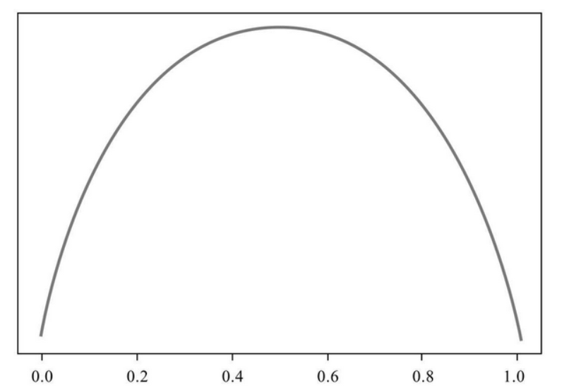
Now let's make these three requirements into images (visual images help to understand them more intuitively). At the same time, if we can find a function that meets this image, we will find a function that meets the conditions. We agree that the horizontal axis of the image represents the proportion of a class and the vertical axis represents the purity value. First, analyze the position of the extreme point.
According to the first requirement, when the proportion of a certain class reaches the maximum and minimum respectively, the purity reaches the highest value. The maximum value is easy to understand. Why can the minimum value also make the purity reach the highest? Conversely, when this class gets the minimum value, another class gets the maximum value, so the purity is the highest. According to the analysis, we know that the purity will reach the maximum at the head and tail of the abscissa.
According to the second requirement, the minimum value of purity occurs when the proportion of a certain class is 50%. In other words, when the abscissa is 0.5, the purity reaches the lowest value.
Now you can make an image. According to the variation of the highest and lowest purity values with the proportion of the class, we connect the three points with a smooth curve, and the image should be similar to a smile curve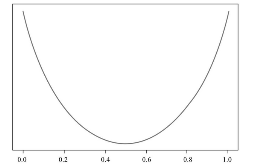
However, we prefer to calculate the "loss value" in machine learning, so the requirements for the purity measurement function are just opposite to those for the purity function, because the lower the purity value, the higher the loss value, and vice versa. So the image produced by the purity measurement function is just the opposite
Background introduction of decision tree algorithm
The earliest decision tree algorithm was CLS proposed by Hunt et al in 1966. Later decision tree algorithms are basically based on the improvement of Hunt algorithm framework.
At present, the most influential decision tree algorithm is ID3 proposed by Quinlan in 1986 and C4 proposed in 1993 5 (now evolved to C5.0), and the CART algorithm proposed by four scholars of BFOS (Breiman, Friedman, Olshen and Stone) in 1984.

Tracing back to its principle, the algorithm principle of decision tree is so clear. The key to establish decision tree is to select which attribute as the classification basis in the current state

Information and quantification of information
Suppose: X is a random variable, xi represents a certain value of X, p(xi) refers to the probability when X=xi, and I(X=xi) represents the amount of information of X=xi
The function satisfies that the greater the probability of an event (the greater the certainty), the smaller the amount of information it carries; on the contrary, the smaller the probability of an event (the smaller the certainty), the greater the amount of information it carries.
1. When a small probability event occurs, we will feel 'a large amount of information'
2. When a high probability event occurs, we will feel 'taken for granted' and 'small amount of information - normal operation'
That is, the more likely an event is to occur, the less information it carries, because there is no need to look for these multiple factors
Information entropy
Entropy: a measure of event uncertainty
Information entropy: in essence, it is a measure of the degree of uncertainty of events, which can also be understood as the average amount of information of an event set

For example, given that Xiaoming's probability of passing is 0.2 and the probability of failing is 0.8, how to measure the uncertainty of Xiaoming's performance?
H (Xiaoming score) = − 0.2 * (log20.2) + (− 0.8 * (log20.8))=0.7219
If the entropy is 0.5, then the probability of failure is 0.5
Conditional entropy
Conditional entropy: it is a concept introduced to explain the information gain, that is, the information entropy of Y under the given condition X. The following is the formula definition:

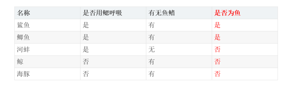
This is a typical dichotomous question: is it a fish
Information entropy: H (fish or not) = - P (FISH) * log2p (FISH) - P (not fish) * log2p (not fish) = - 2/5*log22/5-3/5*log23/5=0.971
Conditional entropy: H (whether fish breathe with gills) = P (breathe with gills) * H (whether fish breathe with gills) + P (breathe without gills) * H (whether fish breathe without gills) = 3/5*(-2/3*log22/3-1/3*log21/3)+2/5(0-1log21)=0.551
H (whether it is a fish or not with fins) = P (with fins) * H (whether it is a fish or not with fins) + P (without fins) * H (whether it is a fish or not with fins) = 4/5*(-1/2*log21/2-1/2*log21/2)+1/5(0-1log21)=0.8
Information Gain (used by ID3 algorithm)
Information gain: the uncertainty of an influencing factor in an event measures the degree to which the uncertainty of event information is reduced, that is, the degree to which the information uncertainty of Class Y is reduced by knowing the information of feature X.
If H(D) is the information entropy of set D and H(D|A) is the conditional entropy of set D under feature A, the information gain can be expressed as the following mathematical formula:

That is, the difference between the information entropy H(D) of set D and the conditional entropy H(D|A) of D under feature A
Strategy of selecting optimal splitting attribute in ID3 algorithm
Firstly, the information entropy H(D) of the current set D before splitting is calculated
Then calculate the conditional entropy H(D|A) of all attributes A contained in the current set D pair
Then calculate the information gain IG(D|A) of each attribute:
IG (D|A)=H(D)−H(D|A)
The attribute AIG=max with the largest information gain is selected as the attribute for splitting the decision tree
Information gain summary
advantage:
1) The two situations of feature occurrence and non occurrence are considered, which is more comprehensive.
2) The statistical attributes of all samples are used to reduce the sensitivity to noise.
3) Easy to understand and simple to calculate.
Disadvantages:
1) Information gain examines the contribution of features to the whole system, not to specific categories, so it can only be used for global feature selection, but not for a single category
2) The algorithm naturally prefers to select attributes with many branches, which is easy to lead to overfitting
Extreme example: if Id is regarded as an attribute, the information gain of ID attribute will be the largest. Because the purest subset can be obtained by dividing the data set according to the ID, that is, the sample of each ID will belong to a single category, so its conditional entropy is 0.
Information gain rate: because the information gain tends to the attribute with the most values, which will lead to over fitting problems, it is necessary to introduce A penalty parameter, that is, the reciprocal of the information entropy of data set D with feature A as the random variable:
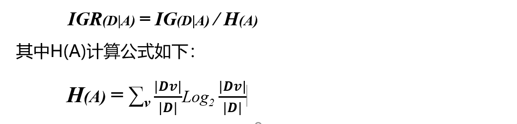
There is A disadvantage opposite to the information gain, that is, it prefers the attribute with the least value, because the smaller the value of attribute A, the smaller the H(A), resulting in the larger IGA(D|A).
Gini index (used by cart algorithm)
Gini index: an index for feature selection similar to information entropy, which can be used to characterize the purity of data. The calculation formula is:

1. Pk indicates the probability that the selected sample belongs to category K, and the probability that it does not belong to category K is (1 − Pk)
2. There are k categories in the sample set. A randomly selected sample can belong to any of these K categories, so the categories are added
3. Gini(p)=2p(1 − p) when it is classified into two categories
Interpretation of Gini index
The smaller the Gini index, the smaller the probability that the selected samples in the set will be wrongly divided, that is, the higher the purity of the set, on the contrary, the impure the set. That is: Gini index (Gini impure) = probability that the sample is selected * probability that the sample is misclassified
Gini index of sample set D: assuming there are K categories in the set, then:

Gini index after dividing sample set D Based on feature A:

Strategy of selecting optimal splitting attribute in CART algorithm
It should be noted that CART is a binary tree, that is, when a feature is used to divide the sample set, there will only be two subsets: 1 A sample set D1 equal to a given eigenvalue; 2. Sample set D2 that is not equal to the given eigenvalue. CART binary tree is actually a binary processing of features with multiple values.
Firstly, for each characteristic attribute A contained in sample set D, A series of binary sets are constructed according to its value
Then calculate the Gini index of the binary set obtained by D Based on each value division of attribute A
Then the attribute value with the smallest Gini index is selected as the optimal partition point
Repeat the above process
code implementation
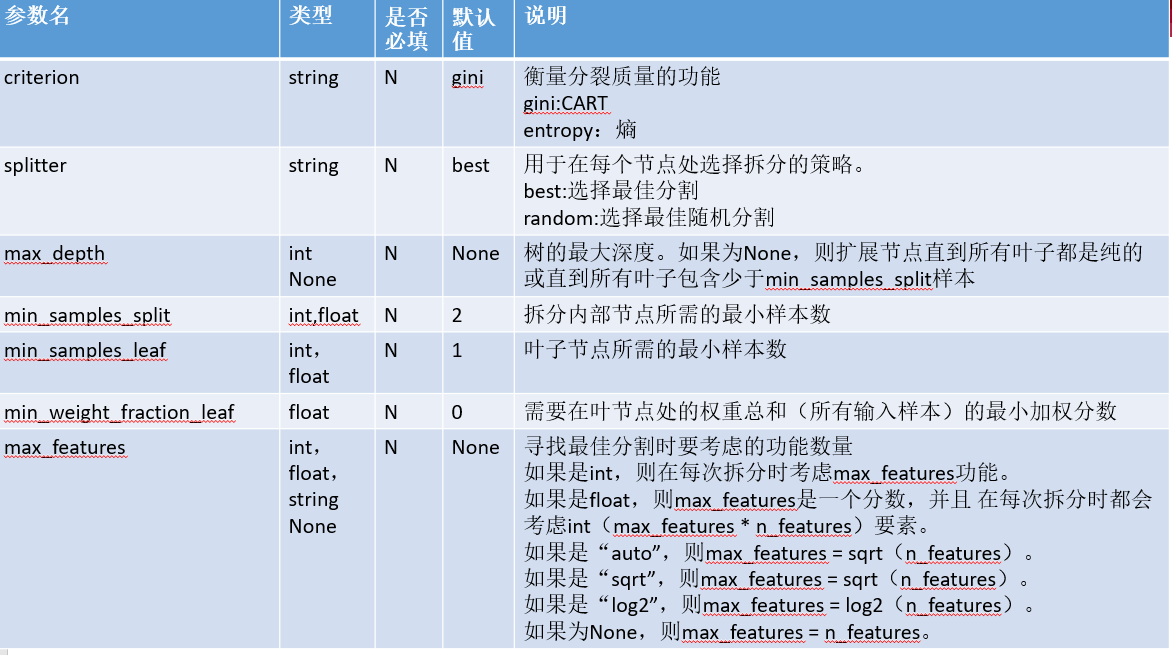
Parameter introduction
sklearn.tree.DecisionTreeClassifier(
	criterion='gini',
	splitter='best',
	max_depth=None,
	min_samples_split=2,
	min_samples_leaf=1,
	min_weight_fraction_leaf=0.0,
	max_features=None,
	random_state=None,
	max_leaf_nodes=None,
	min_impurity_decrease=0.0,
	min_impurity_split=None,
	class_weight=None,
	presort=False)
Importance of characteristics
In the earlier stage, we also introduced the importance of feature selection. For details, click the following article to view the detailed explanation:
Univariate statistics, model-based selection and iterative selection of feature selection
clf.feature_importances_ After returning the importance of the feature, you can use the decision tree to select the feature
Through repeated tests and iterations, I found that selecting the number of features in the decision tree can effectively improve the effect of the model and various evaluation indicators. The previous KNN algorithm interferes with the effect of the model after we pass the feature selection, but the decision tree is different.
Machine learning requires flexible changes, not necessarily according to a fixed thinking. For example, must the parameters searched by the grid be perfect? Not necessarily. Sometimes the parameters manually adjusted are better than grid search, because grid search generally adds some unnecessary parameters.
Parameter splitter
- splitter is also used to control random options in the decision tree. There are two input values:
- Enter "best". Although the decision tree branches randomly, it will give priority to the more important features for branching (the importance can be viewed through the attribute feature_imports_)
- If you enter "random", the decision tree will be more random when branching, the tree will be deeper and larger because it contains more unnecessary information, and the fitting of the training set will be reduced because of these unnecessary information. This is also a way to prevent over fitting.
- When you predict that your model will be over fitted, use splitter and random_state these two parameters to help you reduce the possibility of over fitting after the tree is built.
Pruning parameters
- Without restriction, a decision tree will grow until the index of impurity is the best, or no more features are available. Such a decision tree is often over fitted, which means that it will perform well in the training set but poorly in the test set. The sample data we collected cannot be completely consistent with the overall situation. Therefore, when a decision tree has too good interpretation of the training data, the rules it finds must contain the noise in the training samples and make it insufficient to fit the unknown data.
- In order to make the decision tree more generalized, we should prune the decision tree. Pruning strategy has a great impact on decision tree, and the correct pruning strategy is the core of optimizing decision tree algorithm. sklearn provides us with different pruning strategies:
- max_depth: limit the maximum depth of the tree and cut off all branches exceeding the set depth
- This is the most widely used pruning parameter, which is very effective in high dimension and low sample size. If the decision tree grows one more layer, the demand for sample size will double, so limiting the depth of the tree can effectively limit over fitting. It is also very practical in the integration algorithm. In actual use, it is recommended to try from = 3 to see the fitting effect, and then decide whether to increase the set depth.
- min_samples_leaf & min_samples_split:
- min_samples_leaf defines that each child node of a node after branching must contain at least min_samples_leaf is a training sample, otherwise the branching will not occur, or the branching will meet the requirement that each child node contains min_samples_leaf occurs in the direction of two samples. General collocation max_depth use. Setting the number of this parameter too small will cause over fitting, and setting it too large will prevent the model from learning data. Generally speaking, it is recommended to start with = 5.
- min_samples_split limit, a node must contain at least min_samples_split training samples, this node is allowed to be branched, otherwise the branching will not occur.
- max_depth: limit the maximum depth of the tree and cut off all branches exceeding the set depth
Code case
Import third party libraries
#Import required packages
from sklearn.metrics import precision_score
from sklearn.model_selection import train_test_split
from sklearn.tree import DecisionTreeClassifier
import numpy as np
import pandas as pd
import matplotlib.pyplot as plt
from matplotlib.colors import ListedColormap
from sklearn.preprocessing import LabelEncoder
from sklearn.metrics import classification_report
from sklearn.model_selection import GridSearchCV #Grid search
import matplotlib.pyplot as plt#visualization
import seaborn as sns#Drawing package
When importing data for the first time, do not add any parameters for training
# Loading model
model = DecisionTreeClassifier()

# Training model
model.fit(X_train,y_train)
# Estimate
y_pred = model.predict(X_test)

'''
Evaluation index
'''
# Find the same number of predictions as the real one
true = np.sum(y_pred == y_test )
print('The number of predicted results is:', true)
print('The number of mispredicted results is:', y_test.shape[0]-true)
# Evaluation index
from sklearn.metrics import accuracy_score,precision_score,recall_score,f1_score,cohen_kappa_score
print('The accuracy of prediction data is: {:.4}%'.format(accuracy_score(y_test,y_pred)*100))
print('The accuracy of prediction data is:{:.4}%'.format(
      precision_score(y_test,y_pred)*100))
print('The recall rate of predicted data is:{:.4}%'.format(
      recall_score(y_test,y_pred)*100))
# print("F1 value of training data is:", f1score_train)
print('Forecast data F1 The value is:',
      f1_score(y_test,y_pred))
print('Forecast data Cohen's Kappa The coefficient is:',
      cohen_kappa_score(y_test,y_pred))
# Print classification Report
print('The classification report of forecast data is:','\n',
      classification_report(y_test,y_pred))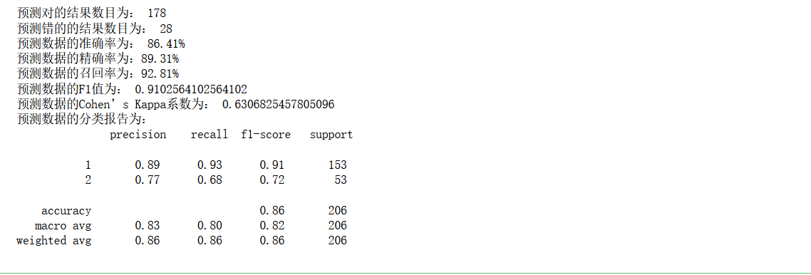
The effect is average, and the following improvement measures are taken
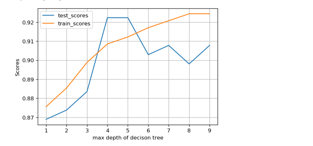
Manually adjust the parameters of max depth
def cv_score(d):
    clf = DecisionTreeClassifier(max_depth=d)
    clf.fit(X_train, y_train)
    return(clf.score(X_train, y_train), clf.score(X_test, y_test))


depths = np.arange(1,10)
scores = [cv_score(d) for d in depths]
tr_scores = [s[0] for s in scores]
te_scores = [s[1] for s in scores]

# Find the index with the highest score in the cross validation dataset
tr_best_index = np.argmax(tr_scores)
te_best_index = np.argmax(te_scores)

print("bestdepth:", te_best_index+1, " bestdepth_score:", te_scores[te_best_index], '\n')

# visualization
%matplotlib inline
from matplotlib import pyplot as plt
depths = np.arange(1,10)
plt.figure(figsize=(6,4), dpi=120)
plt.grid()
plt.xlabel('max depth of decison tree')
plt.ylabel('Scores')
plt.plot(depths, te_scores, label='test_scores')
plt.plot(depths, tr_scores, label='train_scores')
plt.legend()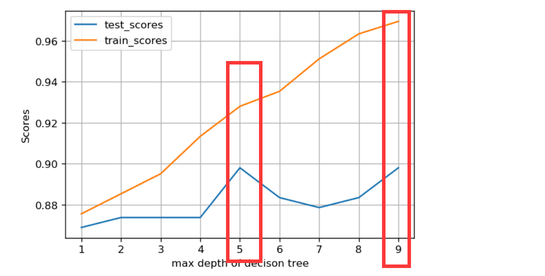
When you get 5 and 9, it looks good, but generally you won't get 9, because it may cause over fitting
The following is an introduction to the idea of tuning one of the parameters
min_impurity_decrease parameter
def minsplit_score(val):
    clf = DecisionTreeClassifier(criterion='gini',max_depth=5, min_impurity_decrease=val)
    clf.fit(X_train, y_train)
    return (clf.score(X_train, y_train), clf.score(X_test, y_test), )


# Specify the parameter range, train the model respectively and calculate the score
vals = np.linspace(0, 0.2, 100)
scores = [minsplit_score(v) for v in vals]
tr_scores = [s[0] for s in scores]
te_scores = [s[1] for s in scores]

bestmin_index = np.argmax(te_scores)
bestscore = te_scores[bestmin_index]
print("bestmin:", vals[bestmin_index])
print("bestscore:", bestscore)

plt.figure(figsize=(6,4), dpi=120)
plt.grid()
plt.xlabel("min_impurity_decrease")
plt.ylabel("Scores")
plt.plot(vals, te_scores, label='test_scores')
plt.plot(vals, tr_scores, label='train_scores')

plt.legend()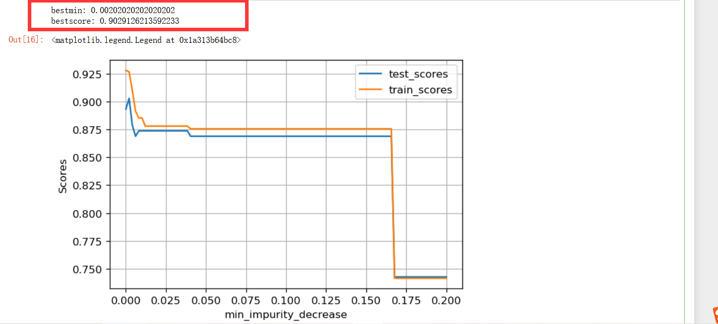
It looks like the effect has improved here
Two main parameters are determined through manual adjustment
Grid search
import numpy as np
from sklearn.model_selection import GridSearchCV

parameters = {'splitter':('best','random')
              ,'criterion':("gini","entropy")
              ,"max_depth":[np.arange(4,10,1)]
              ,"max_depth":[*range(1,10)]
              ,'min_samples_leaf':[*range(1,50,5)]
}

clf = DecisionTreeClassifier(random_state=25)
GS = GridSearchCV(clf, parameters, cv=5) # cv cross validation
GS.fit(X_train,y_train)
GS.best_params_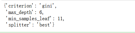
Several main parameters are determined
Bring in the best parameters for training
# Loading model
model = DecisionTreeClassifier(criterion='gini',max_depth=5, splitter= 'random')

# Training model
model.fit(X_train,y_train)
# Estimate
y_pred = model.predict(X_test)

'''
Evaluation index
'''
# Find the same number of predictions as the real one
true = np.sum(y_pred == y_test )
print('The number of predicted results is:', true)
print('The number of mispredicted results is:', y_test.shape[0]-true)
# Evaluation index
from sklearn.metrics import accuracy_score,precision_score,recall_score,f1_score,cohen_kappa_score
print('The accuracy of prediction data is: {:.4}%'.format(accuracy_score(y_test,y_pred)*100))
print('The accuracy of prediction data is:{:.4}%'.format(
      precision_score(y_test,y_pred)*100))
print('The recall rate of predicted data is:{:.4}%'.format(
      recall_score(y_test,y_pred)*100))
# print("F1 value of training data is:", f1score_train)
print('Forecast data F1 The value is:',
      f1_score(y_test,y_pred))
print('Forecast data Cohen's Kappa The coefficient is:',
      cohen_kappa_score(y_test,y_pred))
# Print classification Report
print('The classification report of forecast data is:','\n',
      classification_report(y_test,y_pred))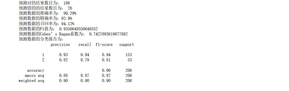
The effect is still average. Generally speaking, it has been improved, but it is not obvious enough and needs to be further improved
Next, we will select features. In the decision tree, feature selection is still very important. Next, we will select features from many aspects to see if it can improve the effect of the model
Feature selection of decision tree model
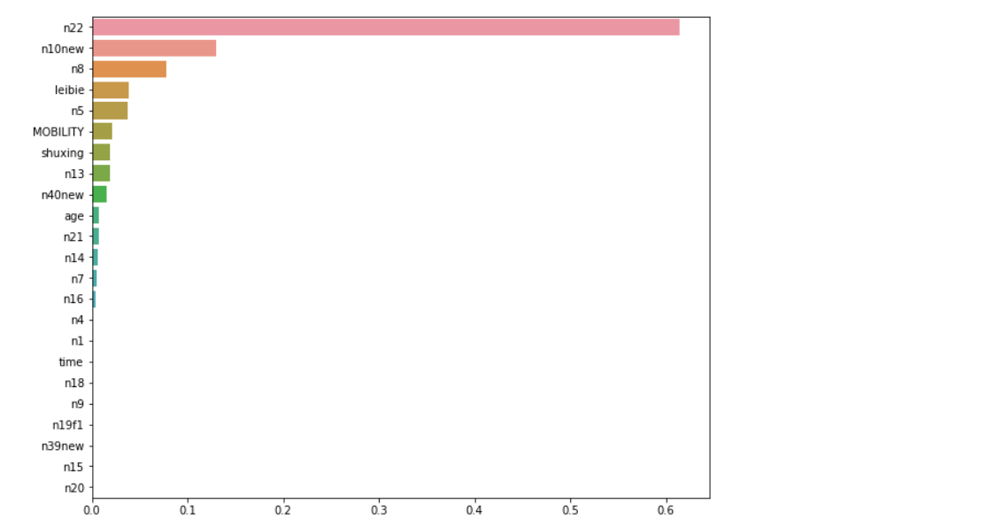
feature_weight = model.feature_importances_
feature_name = df.columns[:-1]
feature_sort = pd.Series(data = feature_weight ,index = feature_name)
feature_sort = feature_sort.sort_values(ascending = False)
plt.figure(figsize=(10,8))
sns.barplot(feature_sort.values,feature_sort.index, orient='h')
Correlation coefficient
plt.subplots(figsize=(10, 15))
sns.heatmap(df.corr()[['n23']].sort_values(by="n23",ascending=False), annot=True, vmax=1, square=True, cmap="Blues")
plt.rcParams['axes.unicode_minus']=False
# plt.rcParams['font.sans-serif']=['HeiTi']
plt.show()
X_name=df.corr()[["n23"]].sort_values(by="n23",ascending=False).iloc[1:7].index.values.astype("U")
print(X_name)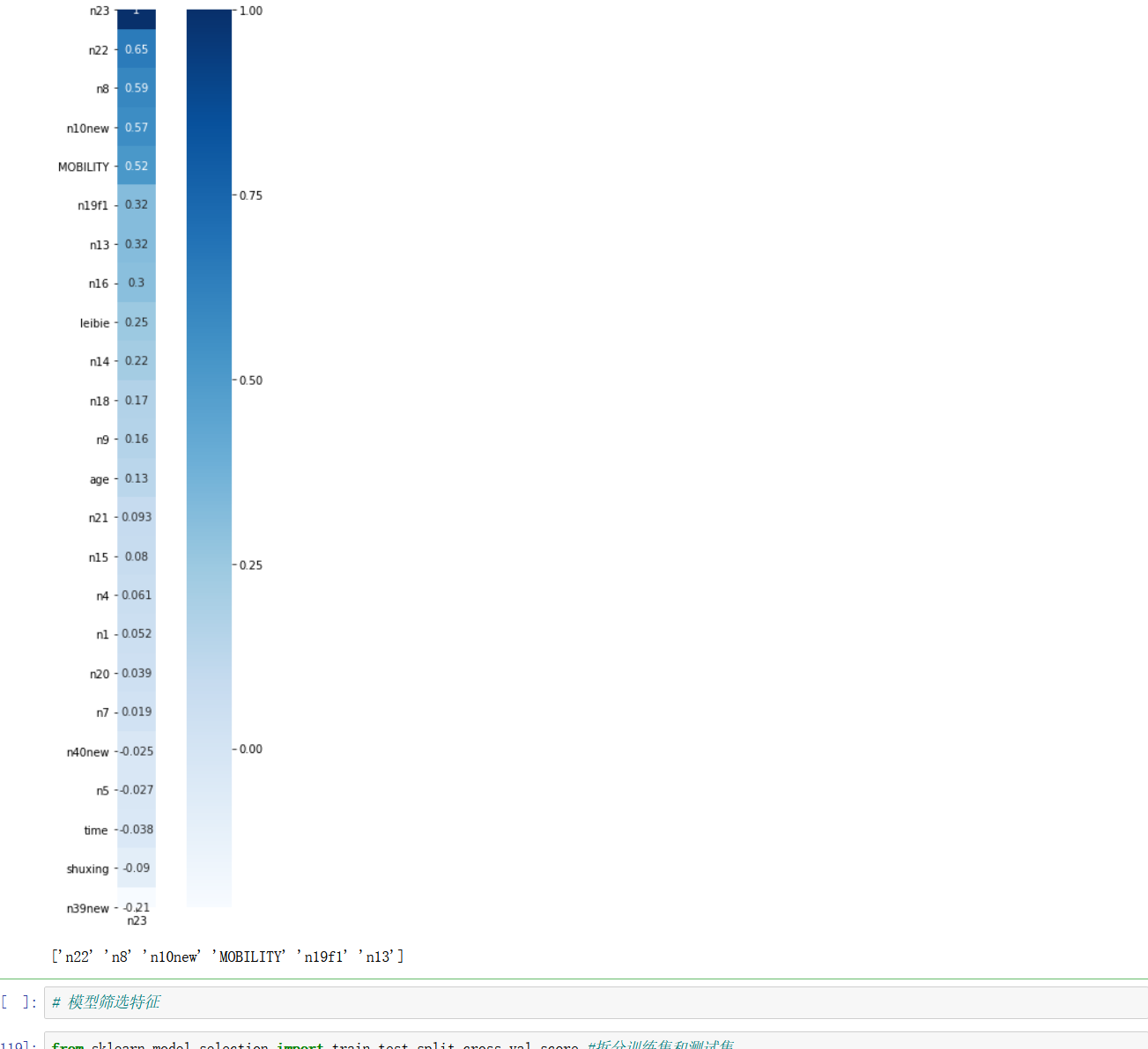
This method is based on the knowledge of mathematical theory, and six important features are selected
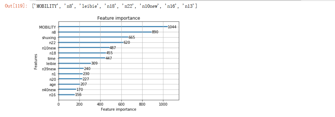
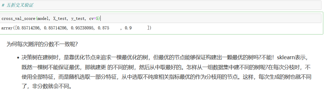
Lightweight and efficient gradient lifting tree feature selection
from sklearn.model_selection import train_test_split,cross_val_score #Split training set and test set
import lightgbm as lgbm #Lightweight and efficient gradient lifting tree

X_train, X_test, y_train, y_test = train_test_split(X,y,test_size=0.2,stratify=y,random_state=1)
lgbm_class = lgbm.LGBMClassifier(max_depth=5,num_leaves=25,learning_rate=0.005,n_estimators=1000,min_child_samples=80, subsample=0.8,colsample_bytree=1,reg_alpha=0,reg_lambda=0)
lgbm_class.fit(X_train, y_train)
#Select the 20 most important features and draw their importance ranking chart
lgbm.plot_importance(lgbm_reg, max_num_features=14)

##You can also not use the built-in plot_importance function, manually obtain the feature importance and feature name, and then draw
feature_weight = lgbm_class.feature_importances_
feature_name = lgbm_class.feature_name_
feature_sort = pd.Series(data = feature_weight ,index = feature_name)
feature_sort = feature_sort.sort_values(ascending = False)
# plt.figure(figsize=(10,8))
# sns.barplot(feature_sort.values,feature_sort.index, orient='h')
lgbm_name=feature_sort.index[:8].tolist()
lgbm_name
Bring in the model again for training
Bring the six features just selected with the correlation coefficient into the model for training, and check the effect again
# Loading model
model = DecisionTreeClassifier(criterion='gini',max_depth=5, splitter= 'random')

# Training model
model.fit(X_train,y_train)
# Estimate
y_pred = model.predict(X_test)

'''
Evaluation index
'''
# Find the same number of predictions as the real one
true = np.sum(y_pred == y_test )
print('The number of predicted results is:', true)
print('The number of mispredicted results is:', y_test.shape[0]-true)
# Evaluation index
from sklearn.metrics import accuracy_score,precision_score,recall_score,f1_score,cohen_kappa_score
print('The accuracy of prediction data is: {:.4}%'.format(accuracy_score(y_test,y_pred)*100))
print('The accuracy of prediction data is:{:.4}%'.format(
      precision_score(y_test,y_pred)*100))
print('The recall rate of predicted data is:{:.4}%'.format(
      recall_score(y_test,y_pred)*100))
# print("F1 value of training data is:", f1score_train)
print('Forecast data F1 The value is:',
      f1_score(y_test,y_pred))
print('Forecast data Cohen's Kappa The coefficient is:',
      cohen_kappa_score(y_test,y_pred))
# Print classification Report
print('The classification report of forecast data is:','\n',
      classification_report(y_test,y_pred))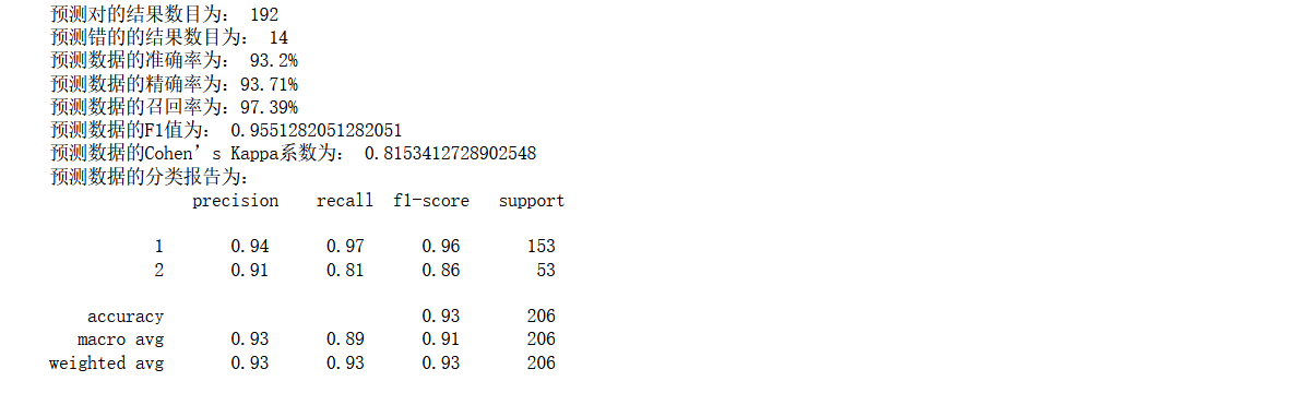
Now it is found that the effect has been significantly improved, the accuracy rate has reached 93%, and the recall rate is relatively high
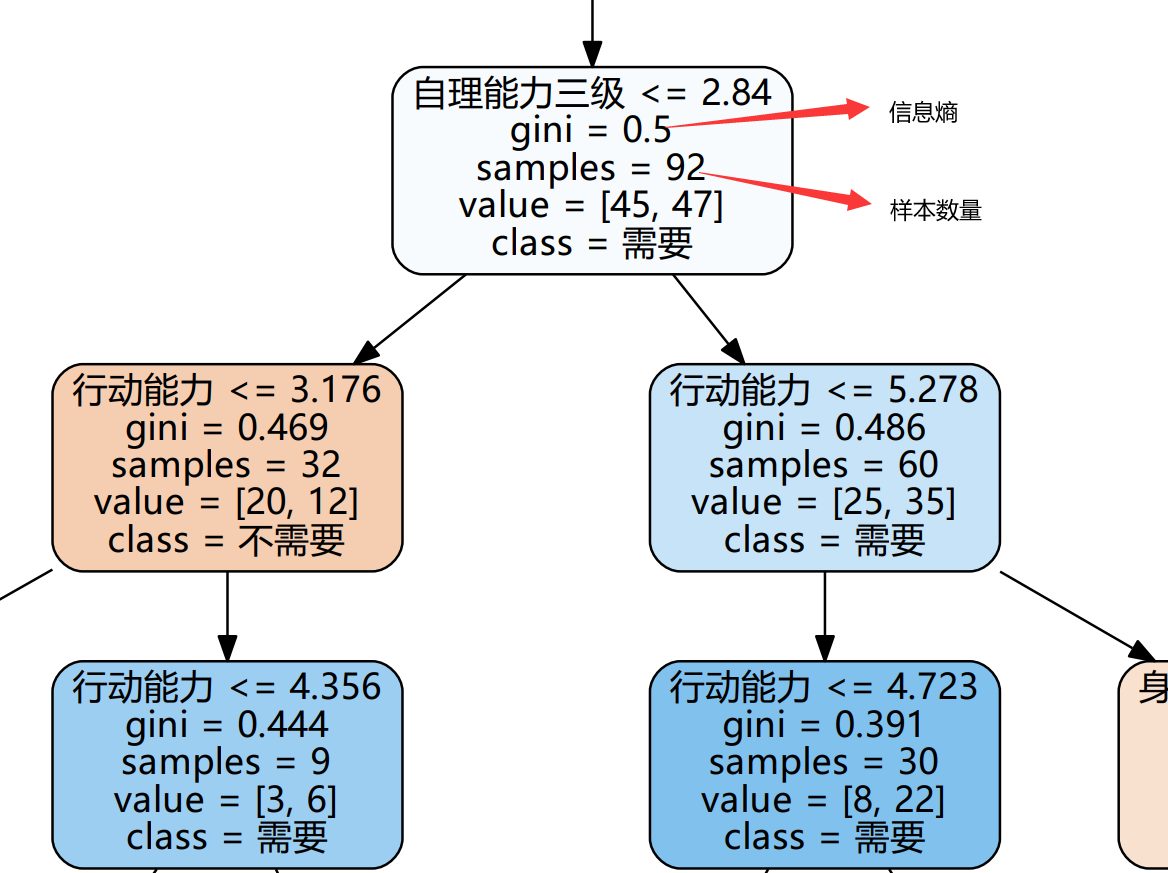
Decision tree visualization
import graphviz
from IPython.display import Image
dot_data = tree.export_graphviz(model
                                ,feature_names= ["Sign informed consent","cognitive function ","Self care ability level III","Action ability","Whether there is pipeline","Physical aggression"]
                                #'n22' 'n8' 'n10new' 'MOBILITY' 'n19f1' 'n13'
                                ,class_names=["unwanted","need"]
                                ,filled=True
                                ,rounded = True
                                ,out_file =None#Picture saving path
                                                               )
graph = graphviz.Source(dot_data.replace('helvetica','"Microsoft YaHei"'), encoding='utf-8')
graph.view()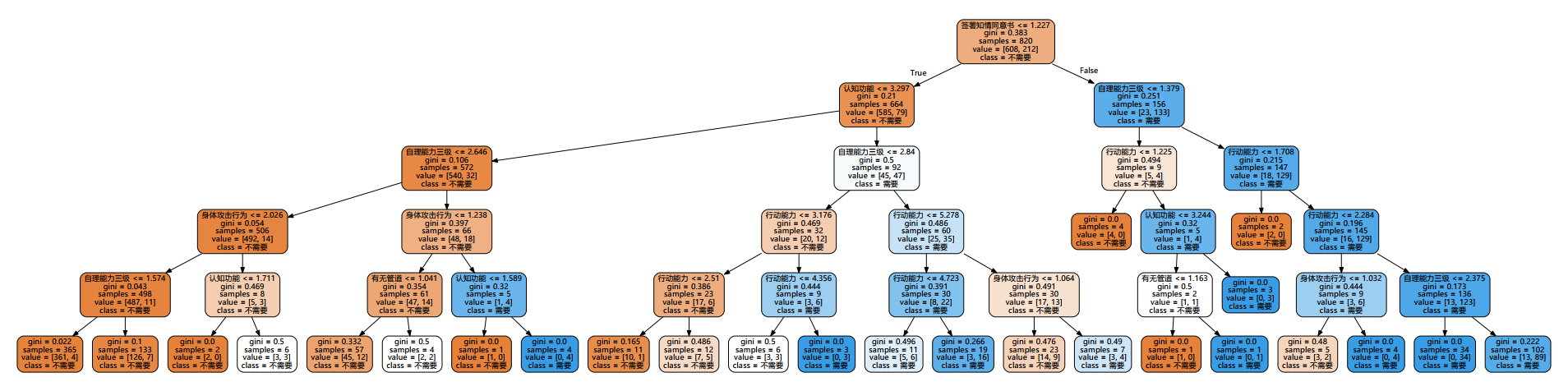
This is the visualization under the decision tree model, which can efficiently show the classification process
ROC curve AUC
from sklearn.metrics import precision_recall_curve
from sklearn import metrics
# Probability of predicting positive cases
y_pred_prob=model.predict_proba(X_test)[:,1]
# y_pred_prob returns two columns. The first column represents category 0 and the second column represents the probability of category 1
#https://blog.csdn.net/dream6104/article/details/89218239
fpr, tpr, thresholds = metrics.roc_curve(y_test,y_pred_prob, pos_label=2)
#pos_label stands for true positive label, which means it is a good label in the classification. It depends on whether your feature target label is 0,1 or 1,2
roc_auc = metrics.auc(fpr, tpr)  #auc is the area under the Roc curve
# print(roc_auc)
plt.figure(figsize=(8,6))
plt.plot([0, 1], [0, 1], color='navy', lw=2, linestyle='--')
plt.plot(fpr, tpr, 'r',label='AUC = %0.2f'% roc_auc)
plt.legend(loc='lower right')
# plt.plot([0, 1], [0, 1], 'r--')
plt.xlim([0, 1.1])
plt.ylim([0, 1.1])
plt.xlabel('False Positive Rate') #The abscissa is fpr
plt.ylabel('True Positive Rate')  #The ordinate is tpr
plt.title('Receiver operating characteristic example')
plt.show()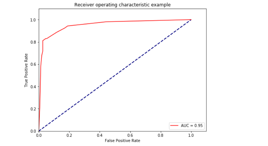
This is the prediction classification under the decision tree. In this model, the model parameters are optimized first, and then the characteristics are selected. Generally speaking, the characteristics should be selected first, and then the parameters are optimized. Through verification, the model effect under this data set is consistent.
The main max depth=5, which is in line with the optimal choice of the model
summary
As mentioned earlier, the parameter controlling the complexity of the decision tree model is the pre pruning parameter, which stops the construction of the tree before the tree is fully expanded. In general, choosing a pre pruning strategy (setting max_depth, max_leaf_nodes, or min_samples_leaf) is sufficient to prevent overfitting.
Compared with many algorithms discussed above, decision tree has two advantages: first, the model is easy to visualize and easy to understand by non experts (at least for small trees); Second, the algorithm is completely unaffected by data scaling. Because each feature is processed separately and the division of data does not depend on scaling, the decision tree algorithm does not need feature preprocessing, such as normalization or standardization. Especially when the scales of features are completely different, or when binary features and continuous features exist at the same time, the effect of decision tree is very good.
The main disadvantage of decision tree is that even if pre pruning is done, it is often over fitted, and the generalization performance is very poor. Therefore, in
In most applications, the subsequent random forest is often used, and the integration method is introduced to replace a single decision tree.
Every word
If you want to pick it up, you should also put it down