catalogue
divide and rule
divide and conquer (D & C) -- a famous recursive problem solving method.
The so-called "divide and conquer" is to divide a complex algorithm problem into equivalent smaller parts according to a certain "decomposition" method, and then solve it one by one, find out the solutions of each part, and form the solutions of each part into the solutions of the whole problem. This simple idea comes from people's life and work experience, and is also completely suitable for the technical field. Such as software architecture design and modular design are the concrete manifestation of divide and rule.
The process of solving problems with D & C includes two steps:
(1) Find the baseline condition (the condition for terminating recursion), which is as simple as possible.
(2) Continue to decompose (or scale down) the problem until it meets the baseline conditions
(3) The solution of the split sub problem is returned layer by layer and merged into the solution of the original problem
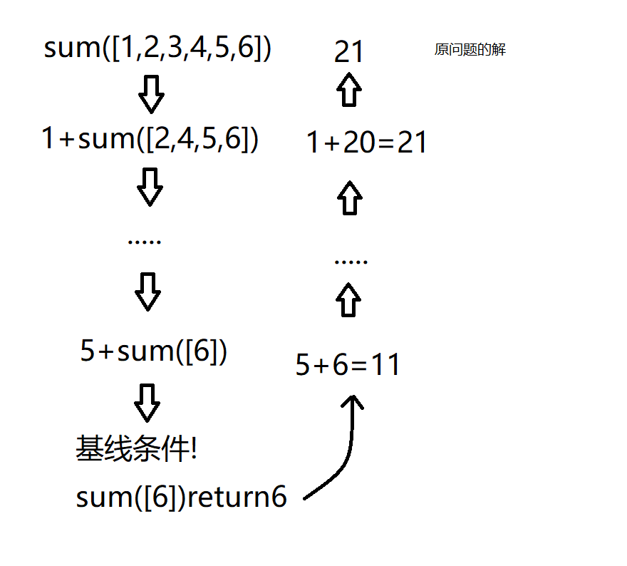
Let's illustrate with an example. Given an array [1,2,3,4,5,6], we need to add these numbers and return their sum. First of all, this problem can be solved by using a for loop, but how to use recursive functions to complete this task?
Step 1: find out the baseline condition, that is, when to stop recursion. I think the array containing one or 0 elements should be terminated
Step 2: reduce the scale of the problem, that is, we have to get closer and closer to the baseline condition every time we recurse.
sum([1,2,3,4,5,6])=21 seems to be equivalent to 1+sum([2,3,4,5,6])=1+20=21, but the scale of the problem seems to be reduced.
Step 3: return the solution of each layer of subproblem and merge it into the solution of the original problem.

python code implementation
def sum(arr):
    """Baseline conditions"""
    if len(arr)<=1:
        return arr[0]
    '''Recursive condition'''
    return arr.pop()+sum(arr)
if __name__ == '__main__':
    arr=[1,2,3,4,5,6]
    print(sum(arr))
This is just an example to illustrate the idea of D & C, but the efficiency of the summation algorithm is not higher than that of the loop, or even worse.
Merge sort
Merge sort is an effective sort algorithm based on merge operation. The algorithm is a very typical application of D & C.
Merge sort method is to merge two (or more) ordered tables into a new ordered table, that is, the sequence to be sorted is divided into several subsequences, and each subsequence is ordered. Then the ordered subsequences are combined into an overall ordered sequence.
Merge the ordered subsequences to obtain a completely ordered sequence; That is, each subsequence is ordered first, and then the subsequence segments are ordered. If two ordered tables are merged into one, it is called 2-way merging. Merge sort is also called merge sort.
For the illustration of merging and sorting, you can read this article Graphical sorting algorithm (4) merge sorting - DREAMCATCHER CX - blog Garden
python code implementation
"""Merge"""
def Merge_sort(arr):
    if len(arr)<=1:
        return arr
    mid=len(arr)//2
    """Recursively divide into two arrays"""
    left=Merge_sort(arr[:mid])
    right=Merge_sort(arr[mid:])
    return Sort(left,right)

"""sort"""
def Sort(a,b):
    c=[]
    while len(a)>0 and len(b)>0:
        """If a First element ratio b If the first element is large, it will b The first element of pops up and adds to the array c In,
        Otherwise, it will a The first element of pops up and is added to the c Medium, when a perhaps b Jump out of loop when any array in is empty"""
        if a[0]>b[0]:
            c.append(b.pop(0))
        else:
            c.append(a.pop(0))
    """If a If the array is empty, the b Add array to c The opposite is the same"""
    if len(a)==0:
        c.extend(b)
    else:
        c.extend(a)
    return c
if __name__ == '__main__':
    a=[2,6,5,20,1,4,22]
    print(Merge_sort(a))
Test results:
[1, 2, 4, 5, 6, 20, 22]
Time complexity
The time complexity of merging and sorting is O(n*logn), and the average and worst cases are O(n*logn). Because its merging time complexity is O(logn) and sorting time complexity is O(n), the total time complexity is O(nlogn).
Quick sort
Quick sort is a commonly used sort algorithm, which is much faster than selective sort. It is not only the optimization of bubble sort algorithm, but also the embodiment of D & C thought.
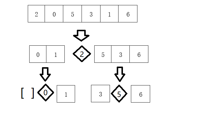
The quick sort algorithm realizes sorting through multiple comparisons and exchanges. The sorting steps are as follows:
(1) Select reference value (pivot)
(2) The array is divided into two sub arrays according to the benchmark value: an array less than the benchmark value and an array greater than the benchmark value
(3) Repeat the above operation for the two sub arrays until the benchmark conditions are met
Let's take the sorting array [2,0,5,3,1,6] as an example. Its steps are as follows

python code implementation
def Quick_sort(arr):
    """Baseline conditions"""
    if len(arr)<1:
        return arr
    pivot=arr[0]#Select reference value
    left=Quick_sort([i for i in arr[1:] if i<pivot])#Less than reference value
    right=Quick_sort([i for i in arr[1:] if i>=pivot])#Greater than reference value
    result=left+[pivot]+right
    return result
if __name__ == '__main__':
    a=[2,0,5,3,1,6]
    print(Quick_sort(a))
Test results:
[0, 1, 2, 3, 5, 6]
Time complexity
The performance of quick sort depends on the benchmark you choose. The time complexity in the average case (optimal case) is O(nlogn), and in the worst case is o( ). If every time we select the first element of the array as the reference value and the array to be sorted is ordered, the number of recursion is n, that is, the height of the call stack is n and the stack length is O(n). Each layer of the call stack involves O(n) elements, so the total time complexity is o(
 ); If every time we choose the middle value of the array as the reference value, the number of recursion is
 , stack length is o(
 ) each layer of the call stack also involves O(n) elements, so the total time complexity is O(nlogn).