%% input data
%% 1602480875@qq.com
%% Version 0.1
clc
clear
close all
S2= xlsread('Formation data.xlsx','Sheet3');
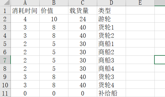
Un = xlsread('Formation data.xlsx','Supply time and value','A1:C10'); % Time consumption of services available amount of substances consumed by time
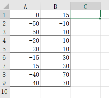
microsoftexcel = xlsread('Formation data.xlsx','Ship coordinates','A1:B9');
qidian_where=[0 0]; %Initial coordinates of supply ship
S3=[microsoftexcel;qidian_where];
%% Clear temporary variables
clearvars raw;
%% Data sorting
xdata=S3;
x_label=xdata(1:end,1);
y_label=xdata(1:end,2);
Demand=Un; %Supply time and value matrix
C=[x_label y_label]; %Coordinate matrix
n=size(C,1); %n Indicates the number of nodes (combat ships)
% ==============Calculate distance matrix==============
D=zeros(n,n); %D The weighted adjacency matrix of a complete graph, that is, the distance matrix D initialization
for i=1:n
for j=1:n
if i~=j
D(i,j)=((C(i,1)-C(j,1))^2+(C(i,2)-C(j,2))^2)^0.5; %Calculate the distance between two ships
if D(i,j)==0
D(i,j)=eps; %Assign a minimum value to a place that cannot be reached directly
end
else
D(i,j)=eps; %i=j, Then the distance is 0; Give a minimum value
end
D(j,i)=D(i,j); %The distance matrix is a symmetric matrix
end
end
v=37; % 30km/h Velocity constraint matrix
Alpha=1;%
Beta=5; %
Rho=0.75; % Information volatility
iter_max=100; %Number of iterations
Q=10; %
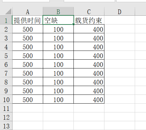
Cap=S2; %Maximum replenishment time limit matrix
m=size(D,1); %Number of initial placement
qidian=m; % qidian Starting point coordinates
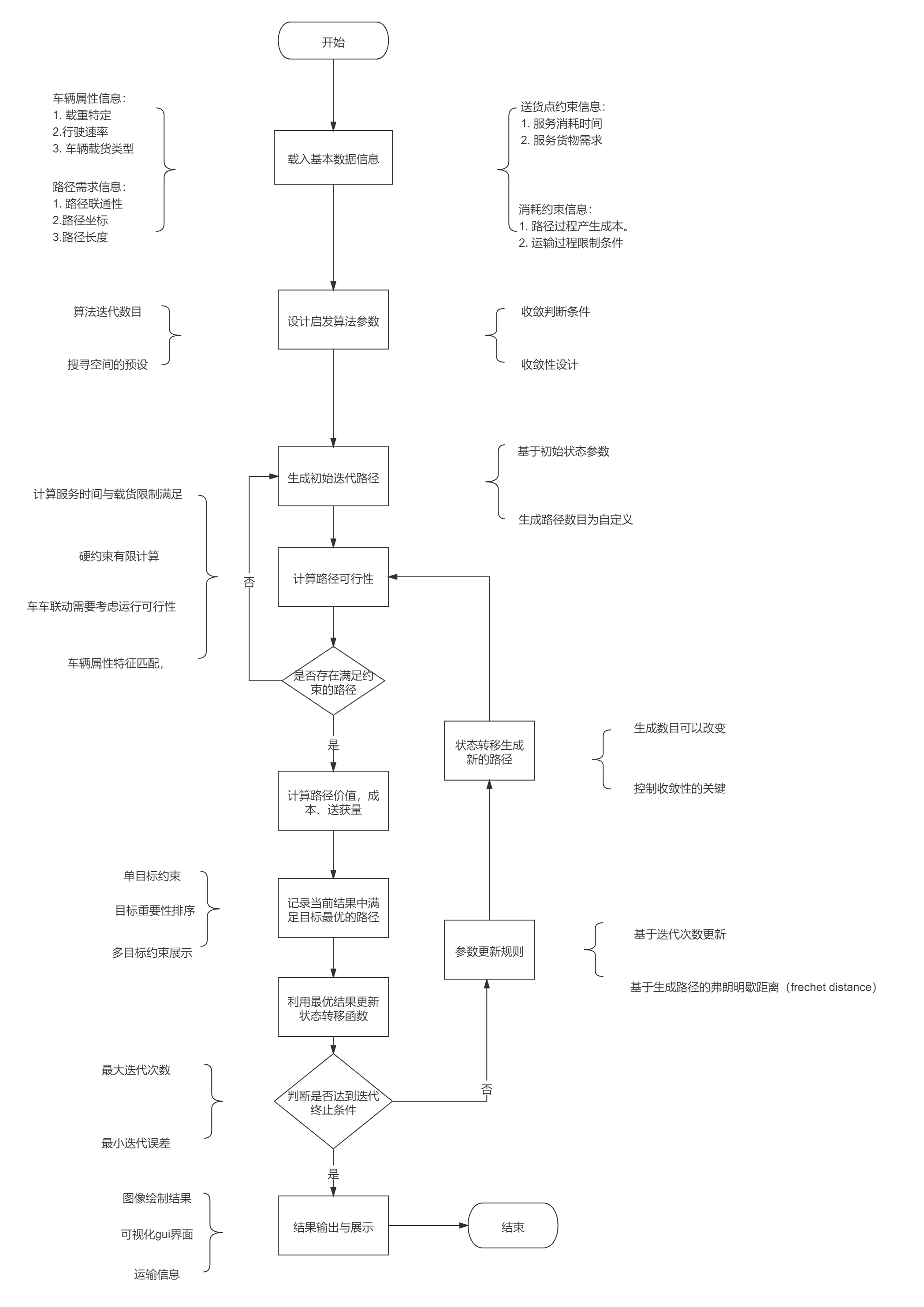
[R_best,L_best,L_ave,Shortest_Route,~,L_ave_long]=ANT_VRP(D,Demand,Cap,iter_max,m,Alpha,Beta,Rho,Q,qidian,v); %Ant colony algorithm VRP Problem constrained function
Shortest_Route_1=Shortest_Route; %Extract the optimal route
cc=find(Shortest_Route_1==qidian);
xx_1=[];
best_route_2=[];
for i=1:length(cc)-1
if i~=length(cc);
cs_1=length(Shortest_Route_1(cc(i):cc(i+1)));
xx_1(i,1:cs_1)=Shortest_Route_1(cc(i):cc(i+1)); %Route
else
end
best_route_1=0;
for j=1:length(xx_1(i,1:cs_1))-1 %Calculate the distance of each path/cost
best_route_1=D(xx_1(i,j),xx_1(i,j+1))+best_route_1;
end
best_route_vaule=0;
for j=1:length(xx_1(i,1:cs_1))-1 %Calculate the distance of each path/cost
best_route_vaule=Demand(xx_1(i,j),2)+best_route_vaule;
end
best_route_2(i,1)= best_route_1; %Length of each path
best_route_2(i,2)= best_route_vaule; %Length of each path
end
[~,n]=max(best_route_2(:,2));
Shortest_Length=best_route_2(n,2); %Extract the shortest path length
%% ==============Mapping==============
figure(1)%Draw iterative convergence curve
x=linspace(0,iter_max,iter_max);
y=L_best(:,1);
plot(x,y);
xlabel('Number of iterations'); ylabel('Maximum supply value');
title('Iterative graph of maximum supply value')
figure(2) %Make the shortest path map
[~,m]=max(best_route_2(:,2));
Shortest_Route=xx_1(m,:);
plot(C(:,1),C(:,2),'*');
hold on
plot(C(Shortest_Route,1),C(Shortest_Route,2),'*-');
axis ( [-60 60 -20 100] ); %Coordinate drawing range
grid on
%% Set import options and import data
S1={'Aircraft carrier','Destroyer 1','Destroyer 2','Frigate 1','Frigate 2','Frigate 3','Frigate 4','Destroyer 3','Destroyer 4','Supply ship'};
for i =1:size(C,1)
% text(C(i,1),C(i,2),[' ' num2str(i)]);
text(C(i,1),C(i,2),[' ' S1(i)]);
end
xlabel('Formation ship abscissa'); ylabel('Longitudinal coordinates of formation ships');
title('Maximum value path map')
figure(3)%Draw iterative convergence curve
axis ( [-60,60,-20,100] );
x=linspace(0,iter_max,iter_max);
y=L_ave_long;
plot(x,y);
xlabel('Number of iterations'); ylabel('Optimal path per generation');
title('Supply route iteration diagram')
xlswrite('Relevant parameters and results.xlsx',[xx_1,best_route_2],'Path results','A2')
clc
beak_length=D(Shortest_Route(end-1),Shortest_Route(end));
all_time=sum(Demand(Shortest_Route))+best_route_2(n,1)/v+beak_length/v;
disp(strcat('Number of iterations:',num2str(iter_max)))
disp(strcat('The maximum replenishment value is:',num2str(Shortest_Length)))
disp(strcat('The maximum supply value path length is:',num2str(best_route_2(n,1))))
disp(strcat('Return path length:',num2str(beak_length)))
disp(strcat('Return path consumption time:',num2str(beak_length/v),'hour'))
disp(strcat('Constraint time:',num2str(S2(1)),'hour'))
disp(strcat('Time remaining:',num2str(S2(1)-all_time),'hour'))
disp(strcat('Remaining service distance:',num2str(v*(S2(1,1)-all_time)),'km'))
disp(strcat('Total elapsed time:',num2str(all_time),'hour'))
disp(strcat('Volume of goods transported:',num2str(sum(Demand(Shortest_Route,3))),'Company'))
disp(strcat('Remaining quantity of transported goods:',num2str(S2(1,3)-sum(Demand(Shortest_Route,3))),'Company'))