1. Trial matrix A = [ 1 2 0 2 0 2 ] A = \begin{bmatrix}1 & 2 & 0\\2 & 0 &2\end{bmatrix} Singular value decomposition of A=[12,20,02].

Solution: I don't think it's necessary to calculate it according to the algorithm flow in the book, understand the theory, and then know how to calculate it. It's nothing more than solving a linear equation, orthogonalizing the eigenvector and other simple linear algebra knowledge.

import numpy as np
def SVD(A):
    U, s, V = np.linalg.svd(A)
    return U, s, V

if __name__ == '__main__':
    A = np.array([[1, 2, 0],
                  [2, 0, 2]])
    U, s, V = SVD(A)
    print('U is :', U)
    print('s is :', s)
    print('V is :', V)

The output is:

U is : [[ 0.4472136  -0.89442719]
 [ 0.89442719  0.4472136 ]]
s is : [3. 2.]
V is : [[ 7.45355992e-01  2.98142397e-01  5.96284794e-01]
 [ 1.94726023e-16 -8.94427191e-01  4.47213595e-01]
 [-6.66666667e-01  3.33333333e-01  6.66666667e-01]]

2. Trial matrix A = [ 2 4 1 3 0 0 0 0 ] A = \begin{bmatrix}2 & 4\\1 & 3\\0 & 0\\0 & 0\end{bmatrix} A = ⎣⎢⎢⎡2100 ⎦⎥⎤ singular value decomposition and write the outer product expression.

import numpy as np
def SVD(A):
    U, s, V = np.linalg.svd(A)
    return U, s, V

if __name__ == '__main__':
    A = np.array([[2, 4],
                  [1, 3],
                  [0, 0],
                  [0, 0]])
    U, s, V = SVD(A)
    print('U is :', U)
    print('s is :', s)
    print('V is :', V)
    #Let's start with the outer product expansion. Here we can calculate 2 or 1, and reduce the rank of the matrix to 1
    B = np.matmul(s[0]*U[:,0:1], V[0:1,:]) + np.matmul(s[1] * U[:, 1:2], V[1:2, :])
    print(A == B)

Output is:

U is : [[-0.81741556 -0.57604844  0.          0.        ]
 [-0.57604844  0.81741556  0.          0.        ]
 [ 0.          0.          1.          0.        ]
 [ 0.          0.          0.          1.        ]]
s is : [5.4649857  0.36596619]
V is : [[-0.40455358 -0.9145143 ]
 [-0.9145143   0.40455358]]
[[ True  True]
 [ True  True]
 [ True  True]
 [ True  True]]

3. Try to compare the similarities and differences between singular value decomposition and diagonalization of symmetric matrix.

Same point: both eigenvalues and eigenvectors need to be calculated
difference:

1. The diagonalization of a symmetric matrix only needs to calculate the eigenvector once, but the matrix composed of the obtained eigenvector may not be an orthogonal matrix, and Schmidt orthogonalization is also needed. Then the orthogonalized vectors are placed according to the position corresponding to the eigenvalue to form an orthogonal matrix. This is where the decomposition is completed.
2. The singular value decomposition of matrix A needs to be calculated first A T A A^TA The eigenvalues of ATA and orthogonal eigenvectors need to square the eigenvalues to form singular values. The orthogonal vectors form V in the order of singular values, and then calculate U according to the relationship between A, U and V A T A^T Orthogonal basis of zero subspace of AT.

4. It is proved that any matrix with rank 1 can write the outer product form of two vectors, and an example is given.

It is proved that let the rank of matrix A be 1
Proof 1: singular value decomposition is not used.
Because the rank of matrix A is 1, we let A = [ A 1 , A 2 , . . . , A n ] A=[A_1, A_2,...,A_n] A=[A1, A2,..., An], because the rank of the matrix is 1, it must exist i 0 i_0 i0 # make A i 0 A_{i_0} Ai0 ， is not a 0 vector.
Rank 1 indicates that n-1 constants can be used c 1 , . . . , c i 0 − 1 , c i 0 + 1 , . . . , c n c_1, ..., c_{i_0 -1}, c_{i_0 + 1}, ...,c_n c1​,..., ci0​−1​,ci0​+1​,..., cn ， multiply A i 0 A_{i_0} Ai0 ， add to No 1 , 2 , . . . , i 0 − 1 , i 0 + 1 , . . . , n 1,2,...,i_0-1, i_0+1,...,n 1,2,...,i0​−1,i0​+1,...,n columns make the elements of these columns of the matrix 0
that is A j = − c j ∗ A i 0 , j = 1 , 2 , . . . , i 0 − 1 , i 0 + 1 , . . . , n A_j = -c_j*A_{i_0}, j = 1,2,...,i_0-1, i_0+1,...,n Aj​=−cj​∗Ai0​​,j=1,2,...,i0​−1,i0​+1,...,n
therefore A = [ − c 1 A i 0 , . . . , − c i 0 − 1 A i 0 , A i 0 , c i 0 + 1 A i 0 , . . . , A n ] = A i 0 ∗ [ − c 1 , . . . , − c i 0 − 1 , 1 , − c i 0 + 1 , . . . , − c n ] A = [-c_1A_{i_0},..., -c_{i_0-1}A_{i_0},A_{i_0},c_{i_0+1}A_{i_0},...,A_n]\\=A_{i_0}*[-c_1, ..., -c_{i_0 -1}, 1,-c_{i_0 + 1}, ...,-c_n] A=[−c1​Ai0​​,...,−ci0​−1​Ai0​​,Ai0​​,ci0​+1​Ai0​​,...,An​]=Ai0​​∗[−c1​,...,−ci0​−1​,1,−ci0​+1​,...,−cn​]
because A i 0 A_{i_0} Ai0 ， is a column vector because it is proved.

Singular value decomposition algorithm 2
Because the rank of matrix A is 1, then using singular value decomposition, we can get
A = U Σ V A = U \Sigma V A=UΣV
Rank 1 Description Σ \Sigma Σ There is only one element in it. The first element is positive and set to a a a. The rest are 0
So according to the expansion of the outer product, we can get A = a U 1 ∗ V 1 T A = aU_1*V_1^T A=aU1​∗V1T​
among U 1 U_1 U1 is the first column of an orthogonal matrix and is a column vector, V 1 V_1 V1 ￠ is the first column of orthogonal matrix V and a vector, which is proved.

5. Singular value decomposition is performed on the click data, and the contents represented by the three matrices are explained.

The recommendation algorithm has been designed here.
The matrix of click data is:
A = [ 0 20 5 0 0 10 0 0 3 0 0 0 0 0 1 0 0 1 0 0 ] A = \begin{bmatrix} 0 & 20 & 5 & 0 & 0\\ 10 & 0 & 0 & 3 & 0\\ 0 & 0 & 0 & 0 & 1\\ 0 & 0 & 1 & 0 &0 \end{bmatrix} A=⎣⎢⎢⎡​01000​20000​5001​0300​0010​⎦⎥⎥⎤​

import numpy as np
def SVD(A):
    U, s, V = np.linalg.svd(A)
    return U, s, V

if __name__ == '__main__':
    A = np.array([[0, 20, 5, 0, 0],
                  [10, 0, 0, 3, 0],
                  [0, 0, 0, 0, 1],
                  [0, 0, 1, 0, 0]])
    U, s, V = SVD(A)
    print('U is :', U)
    print('s is :', s)
    print('V is :', V)

The output is:

U is : [[ 9.99930496e-01 -1.01352447e-16  0.00000000e+00 -1.17899939e-02]
 [ 0.00000000e+00  1.00000000e+00  0.00000000e+00 -8.65973959e-15]
 [ 0.00000000e+00  0.00000000e+00  1.00000000e+00  0.00000000e+00]
 [ 1.17899939e-02  8.65973959e-15  0.00000000e+00  9.99930496e-01]]
s is : [20.61695792 10.44030651  1.          0.97007522]
V is : [[ 0.00000000e+00  9.70007796e-01  2.43073808e-01  0.00000000e+00
   0.00000000e+00]
 [ 9.57826285e-01 -2.31404926e-16  8.02571613e-16  2.87347886e-01
   0.00000000e+00]
 [-0.00000000e+00  0.00000000e+00  0.00000000e+00  0.00000000e+00
   1.00000000e+00]
 [-7.97105437e-16 -2.43073808e-01  9.70007796e-01  0.00000000e+00
   0.00000000e+00]
 [ 2.87347886e-01 -1.01402229e-16  2.10571835e-16 -9.57826285e-01
   0.00000000e+00]]

First, explain matrix V

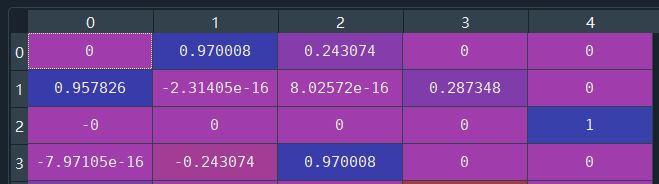
We regard each column as a URL, because the fifth singular value is 0. According to the outer product form, the fifth row is not needed directly. The features of the second dimension of URL1 represented by the first column are more significant, the features of the first position of URL2 represented by the first column are more significant, and the fourth feature of URL3 represented by the third column is more significant. We will distinguish which URL q will tend to click according to the matrix U, that is, when the user enters a query, The recommendation system should first recommend which URL link to the user.

Matrix U is explained below

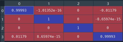
Each column of U is regarded as a query. The first query q1 tends to the URL with more significant characteristics of the first dimension. Looking at the V matrix above, we can see that the characteristics of the first dimension of URL2 are more significant. Therefore, when inputting query q1, the recommendation system should first recommend URL2 to the user, which also explains why the number of clicks of query q1 on URL2 is 20. The second column of U is q2, which is biased towards the URL with larger characteristics. Looking at V above, it is found that the characteristics of the second position of URL1 are more significant. When entering q2, click URL1 up to 10 times.
Here are singular values

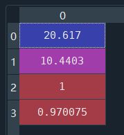
It can be regarded as the importance of each feature of the URL. You can see that the first two are more important.