1. Introduction to Random sample consensus (RANSAC) theory

Ordinary LS is conservative: how to achieve the best under the existing data. It is to consider from the perspective of minimizing the overall error and try not to offend anyone.

RANSAC is a reformist: first, assume that the data has some characteristics (purpose), and appropriately give up some existing data in order to achieve the purpose.

The fitting comparison of least square fitting (red line) and RANSAC (green line) for first-order straight line and second-order curve is given:

It can be seen that RANSAC can fit well. RANSAC can be understood as a way of sampling, so it is theoretically applicable to polynomial fitting, Gaussian mixture model (GMM), etc.

RANSAC's algorithm can be roughly expressed as (from wikipedia):

Given:
data – a set of observed data points
model – a model that can be fitted to data points
n – the minimum number of data values required to fit the model
k – the maximum number of iterations allowed in the algorithm
t – a threshold value for determining when a data point fits a model
d – the number of close data values required to assert that a model fits well to data

Return:
bestfit – model parameters which best fit the data (or nul if no good model is found)

iterations = 0
bestfit = nul
besterr = something really large
while iterations < k {
maybeinliers = n randomly selected values from data
maybemodel = model parameters fitted to maybeinliers
alsoinliers = empty set
for every point in data not in maybeinliers {
if point fits maybemodel with an error smaller than t
add point to alsoinliers
}
if the number of elements in alsoinliers is > d {
% this implies that we may have found a good model
% now test how good it is
bettermodel = model parameters fitted to all points in maybeinliers and alsoinliers
thiserr = a measure of how well model fits these points
if thiserr < besterr {
bestfit = bettermodel
besterr = thiserr
}
}
increment iterations
}
return bestfit
The idea of RANSAC simplified version is:
Step 1: assume the model (such as linear equation), and randomly select Nums sample points (taking 2 as examples) to fit the model:

Step 2: since it is not strictly linear, the data points fluctuate to a certain extent. Assuming that the tolerance range is sigma, find out the points within the tolerance range of the distance fitting curve and count the number of points:

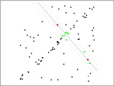
Step 3: re select Nums points randomly and repeat the operations from step 1 to step 2 until the iteration is completed:

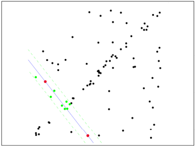
Step 4: after each fitting, there are corresponding data points within the tolerance range. Find out the case with the largest number of data points, which is the final fitting result:

So far: the simplified version of RANSAC has been solved.

This simplified version of RANSAC is only given the number of iterations, and the optimal solution is found at the end of the iteration. If the number of samples is very large, is it difficult to iterate all the time? In fact, RANSAC ignores several problems:

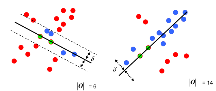
Number of random samples per time Nums Selection of: for example, the conic needs at least 3 points to be determined. Generally speaking, Nums Less is easy to get better results;
Sampling iteration times Iter Selection of: that is, how many times the extraction is repeated, it is considered to meet the requirements and stop the operation? Too much computation and too little performance may not be ideal;
tolerance Sigma Selection of: sigma Taking the big and the small will have a great impact on the final result;

For details of these parameters, refer to: Wikipedia

The function of RANSAC is a bit similar: all the data are divided into two sections, one is our own, the other is the enemy. Our own people stay to discuss things, and the enemy drives them out. RANSAC holds family meetings, unlike least squares, which always holds plenary meetings.

2. Random sample consensus (RANSAC) program implementation

Attach the code of first-order straight line and second-order curve fitting (just to illustrate the most basic idea, the simplified version of RANSAC is used):

First order straight line fitting:

clc;clear all;close all;
 set(0,'defaultfigurecolor','w');
%Generate data
param = [3 2];
npa = length(param);
x = -20:20;
y = param*[x; ones(1,length(x))]+3*randn(1,length(x));
data = [x randi(20,1,30);...
    y randi(20,1,30)];
%figure
figure
subplot 221
plot(data(1,:),data(2,:),'k*');hold on;
%Ordinary least square mean
p = polyfit(data(1,:),data(2,:),npa-1);
flms = polyval(p,x);
plot(x,flms,'r','linewidth',2);hold on;
title('Least square fitting');
%Ransac
Iter = 100;
sigma = 1;
Nums = 2;%number select
res = zeros(Iter,npa+1);
for i = 1:Iter
idx = randperm(size(data,2),Nums);
if diff(idx) ==0
    continue;
end
sample = data(:,idx);
pest = polyfit(sample(1,:),sample(2,:),npa-1);%parameter estimate
res(i,1:npa) = pest;
res(i,npa+1) = numel(find(abs(polyval(pest,data(1,:))-data(2,:))<sigma));
end
[~,pos] = max(res(:,npa+1));
pest = res(pos,1:npa);
fransac = polyval(pest,x);
%figure
subplot 222
plot(data(1,:),data(2,:),'k*');hold on;
plot(x,flms,'r','linewidth',2);hold on;
plot(x,fransac,'g','linewidth',2);hold on;
title('RANSAC');

Second order curve fitting:

clc;clear all;
 set(0,'defaultfigurecolor','w');
%Generate data
param = [3 2 5];
npa = length(param);
x = -20:20;
y = param*[x.^2;x;ones(1,length(x))]+3*randn(1,length(x));
data = [x randi(20,1,30);...
    y randi(200,1,30)];
%figure
subplot 223
plot(data(1,:),data(2,:),'k*');hold on;
%Ordinary least square mean
p = polyfit(data(1,:),data(2,:),npa-1);
flms = polyval(p,x);
plot(x,flms,'r','linewidth',2);hold on;
title('Least square fitting');
%Ransac
Iter = 100;
sigma = 1;
Nums = 3;%number select
res = zeros(Iter,npa+1);
for i = 1:Iter
idx = randperm(size(data,2),Nums);
if diff(idx) ==0
    continue;
end
sample = data(:,idx);
pest = polyfit(sample(1,:),sample(2,:),npa-1);%parameter estimate
res(i,1:npa) = pest;
res(i,npa+1) = numel(find(abs(polyval(pest,data(1,:))-data(2,:))<sigma));
end
[~,pos] = max(res(:,npa+1));
pest = res(pos,1:npa);
fransac = polyval(pest,x);
%figure
subplot 224
plot(data(1,:),data(2,:),'k*');hold on;
plot(x,flms,'r','linewidth',2);hold on;
plot(x,fransac,'g','linewidth',2);hold on;
title('RANSAC');

reference resources:
1: https://en.wikipedia.org/wiki/Random_sample_consensus
2: http://www.cnblogs.com/xingshansi/p/6763668.html