Learning latent variables using self encoder
Because there are many redundancies in the high-dimensional input space, it can be compressed into some low-dimensional variables. The self encoder was first introduced by Geoffrey Hinton et al. In the 1980s. Similar to the technology used to reduce the input dimension in traditional machine learning technology, such as principal component analysis (PCA).
However, in image generation, we also want to restore the low-dimensional space to the high-dimensional space. It can be regarded as image compression, in which the original image is compressed into a file format such as JPEG, which is small and easy to store and transmit. The computer can then restore the JPEG to its original pixels. In other words, the original pixels are compressed into low dimensional JPEG format and restored to high dimensional original pixels for display.
Self coder is an unsupervised machine learning technology, which can train the model without training label. However, because we really need to use the image itself as a label, it is called self supervised machine learning (auto is self in Latin).
The basic building blocks of self encoder are encoder and decoder. The encoder is responsible for reducing the high-dimensional input to some low-dimensional latent (implicit) variables. The decoder is a module that converts hidden variables back to high-dimensional space. The encoder decoder architecture is also used in other machine learning tasks, such as semantic segmentation, in which the neural network first understands the image representation and then generates pixel level labels. The following figure shows the general architecture of the self encoder:
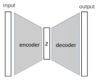
The input and output are images of the same dimension, and z is the latent vector of low dimension. The encoder compresses the input to z and the decoder processes the reverse to generate the output image.
encoder
The encoder is composed of multiple neural network layers. We will use MNIST data set to build the encoder. The input size accepted by the encoder is 28x28x1. We need to set the dimension of latent variable. Here we use one-dimensional vector. The size of the latent variable should be less than the input size. It is a super parameter. First try to use 10, which has a compression ratio of 28 * 28 / 10 = 78.4.
This network extension enables the model to learn important knowledge, discard secondary features layer by layer, and finally get 10 most important features. It looks very similar to CNN classification, in which the size of feature map gradually decreases from top to bottom.
Using convolution layer to build encoder, CNN (such as VGG) in the early stage uses maximum pooling for feature map down sampling, but newer networks tend to achieve this purpose by using convolution with step of 2 in convolution layer.
We will follow the Convention and name the potential variable z:
def Encoder(z_dim):
    inputs  = layers.Input(shape=[28,28,1])
    x = inputs
    x = Conv2D(filters=8, kernel_size=(3,3), strides=2, padding='same', activation='relu')(x)
    x = Conv2D(filters=8, kernel_size=(3,3), strides=1, padding='same', activation='relu')(x)
    x = Conv2D(filters=8, kernel_size=(3,3), strides=2, padding='same', activation='relu')(x)
    x = Conv2D(filters=8, kernel_size=(3,3), strides=1, padding='same', activation='relu')(x)
    x = Flatten()(x)
    out = Dense(z_dim, activation='relu')(x)
    return Model(inputs=inputs, outputs=out, name='encoder')
In a typical CNN architecture, the number of filters increases and the size of the feature map decreases. However, our goal is to reduce the feature size, so the number of filters remains unchanged, which is sufficient for simple data such as MNIST. Finally, we flatten the output of the last convolution layer and feed it to the dense layer to output the latent variable.
decoder
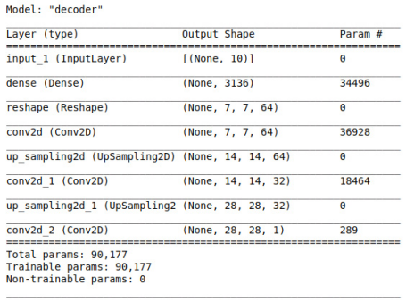
The work of the decoder is essentially opposite to that of the encoder, which converts low-dimensional latent variables into high-dimensional output to approximate the input image. Here, the convolution layer is used in the decoder to sample the characteristic map from 7x7 to 28x28:
def Decoder(z_dim):
    inputs = layers.Input(shape=[z_dim])
    x = inputs
    x = Dense(7*7*64, activation='relu')(x)
    x = Reshape((7,7,64))(x)
    x = Conv2D(filters=64, kernel_size=(3,3), strides=1, padding='same', activation='relu')(x)
    x = UpSampling2D((2,2))(x)
    x = Conv2D(filters=32, kernel_size=(3,3), strides=1, padding='same', activation='relu')(x)
    x = UpSampling2D((2,2))(x)
    x = Conv2D(filters=32, kernel_size=(3,3), strides=2, padding='same', activation='relu')(x)
    out = Conv2(filters=1, kernel_size=(3,3), strides=1, padding='same', activation='sigmoid')(x)
    return Model(inputs=inputs, outputs=out, name='decoder')
Different from the encoder, the purpose of the decoder is not to reduce the size, so we should use more filters to give it more powerful generation ability.
UpSampling2D interpolates pixels to improve resolution. This is an affine transformation (linear multiplication and addition), so it can be back propagated, but it uses fixed weights, so it is not trainable. Another popular upsampling method is to use a transpose convolutional layer, which is trainable, but it may create a similar image in the generated image Artifacts of checkerboard squares.
The convolution model tends not to use the nearest image
Build self encoder
Put the encoder and decoder together to create a self encoder. First, we instantiate the encoder and decoder respectively. Then, we feed the output of the encoder into the input of the decoder, and instantiate a Model using the input of the encoder and the output of the decoder:
z_dim = 10
encoder = Encoder(z_dim)
decoder = Decoder(z_dim)
model_input = encoder.input
model_output = decoder(encoder.output)
autoencoder = Model(model_input, model_output)
For training, L2 loss is used, which is achieved by comparing each pixel between the output and the expected result through mean square error (MSE). In this example, some callback functions are added, which will be called after training each epoch:
- ModelCheckpoint(monitor = 'val_loss') is used to save the model when the current verification loss is lower than the previous epoch.
- If the verification loss is not improved within 10 epoch s, EarlyStopping(monitor = 'val_loss', patience = 10) can stop training earlier.
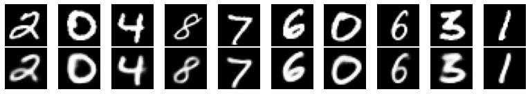
The generated image is as follows:
Generating images from latent variables
So, what is the use of automatic encoder? One of the applications of self encoder is image denoising, that is, adding some noise to the input image and training the model to generate a clear image.
If you are interested in generating images using a self encoder, you can ignore the encoder and use only the decoder to sample from latent variables to generate images. The first challenge we face is to determine how to sample from potential variables.
For illustration, use z_dim = 2 trains another automatic encoder so that we can explore potential space in two dimensions:
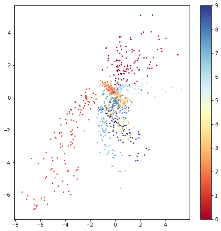
The plot is generated by passing 1000 samples to a trained encoder and drawing two potential variables on the scatter plot. The color bar on the right indicates the strength of the digital label. We can observe from the figure:
The categories of potential variables are not evenly distributed. Clusters that are completely separate from other categories can be seen in the upper left and right. However, the categories at the center of the graph tend to be arranged more densely and overlap each other.
In the following figure, these images are generated in the range of latent variables [- 5, + 5] at intervals of 1.0:
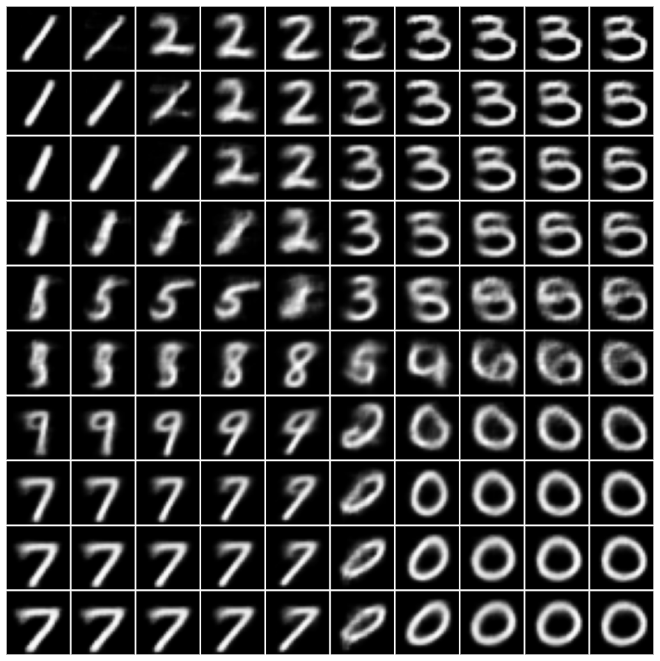
We can see that the numbers 0 and 1 are well represented in the sample distribution and drawn well. But the numbers in the middle are vague, and even some numbers are missing from the sample.
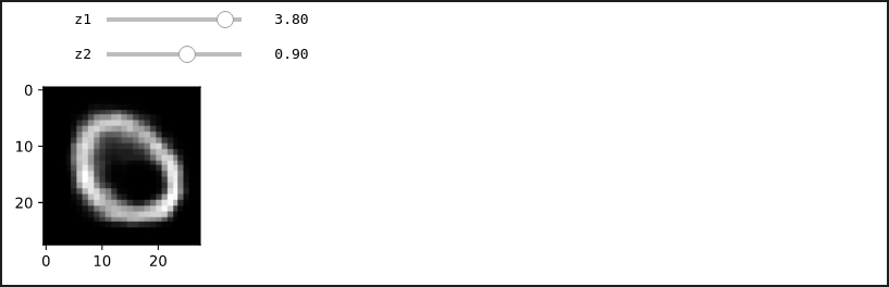
There is a widget in ipynb code that allows sliding to change latent variables to generate images interactively.
Complete code
# autoencoder.ipynb
import tensorflow as tf
from tensorflow.keras import layers, Model
from tensorflow.keras.layers import Input, Conv2D, Dense,\
    Flatten, Reshape, Conv2DTranspose, MaxPooling2D, UpSampling2D, \
        LeakyReLU
from tensorflow.keras.activations import relu
from tensorflow.keras.models import Sequential, load_model
from tensorflow.keras.callbacks import ModelCheckpoint, EarlyStopping

import tensorflow_datasets as tfds

import numpy as np
import matplotlib.pyplot as plt

import warnings
warnings.filterwarnings('ignore')
print(tf.__version__)

(ds_train, ds_test_), ds_info = tfds.load(
    'mnist',
    split=['train','test'],
    shuffle_files=True,
    as_supervised=True,
    with_info=True
)
fig = tfds.show_examples(ds_train,ds_info)

batch_size = 64
def preprocess(image, label):
    image = tf.cast(image, tf.float32)
    image = image/255.
    return image, image

ds_train = ds_train.map(preprocess)
ds_train = ds_train.cache() #put dataset input memory
ds_train = ds_train.shuffle(ds_info.splits['train'].num_examples)
ds_train = ds_train.batch(batch_size,drop_remainder=True)

ds_test = ds_test_.map(preprocess).batch(batch_size,drop_remainder=True).cache().prefetch(batch_size)

# return label for testing
def preprocess_with_label(image, label):
    image = tf.cast(image, tf.float32)
    image = tf.math.round(image/255.)
    return image, label

ds_test_label = ds_test_.map(preprocess_with_label).batch(1000, drop_remainder=True)

def Encoder(z_dim):
    inputs  = layers.Input(shape=[28,28,1])

    x = inputs
    x = Conv2D(filters=8,  kernel_size=(3,3), strides=2, padding='same', activation='relu')(x)
    x = Conv2D(filters=8,  kernel_size=(3,3), strides=1, padding='same', activation='relu')(x)
    x = Conv2D(filters=8,  kernel_size=(3,3), strides=2, padding='same', activation='relu')(x)
    x = Conv2D(filters=8,  kernel_size=(3,3), strides=1, padding='same', activation='relu')(x)
    x = Flatten()(x)
    out = Dense(z_dim)(x)

    return Model(inputs=inputs, outputs=out, name='encoder')

def Decoder(z_dim):
    inputs  = layers.Input(shape=[z_dim])
    x = inputs
    x = Dense(7*7*64, activation='relu')(x)
    x = Reshape((7,7,64))(x)

    x = Conv2D(filters=64, kernel_size=(3,3), strides=1, padding='same', activation='relu')(x)
    x = UpSampling2D((2,2))(x)

    x = Conv2D(filters=32, kernel_size=(3,3), strides=1, padding='same', activation='relu')(x)
    x = UpSampling2D((2,2))(x)

    out = Conv2D(filters=1, kernel_size=(3,3), strides=1, padding='same', activation='sigmoid')(x)

    #return out
    return Model(inputs=inputs, outputs=out, name='decoder')

class Autoencoder:
    def __init__(self, z_dim):
        self.encoder = Encoder(z_dim)
        self.decoder = Decoder(z_dim)

        model_input = self.encoder.input
        model_output = self.decoder(self.encoder.output)
        self.model = Model(model_input, model_output)

autoencoder = Autoencoder(z_dim=10)
model_path = 'autoencoder.h5'
checkpoint = ModelCheckpoint(model_path,
                             monitor= "val_loss",
                             verbose=1,
                             save_best_only=True,
                             mode= "auto",
                             save_weights_only = False)

early = EarlyStopping(monitor= "val_loss",
                      mode= "auto",
                      patience = 5)

callbacks_list = [checkpoint, early]

autoencoder.model.compile(
    loss='mse',
    optimizer=tf.keras.optimizers.RMSprop(learning_rate=3e-4),
    # metrics=[tf.keras.losses.BinaryCrossentropy()]
)
autoencoder.model.fit(ds_train, validation_data=ds_test,
                epochs = 100, callbacks = callbacks_list)

images, labels = next(iter(ds_test))
autoencoder.model = load_model(model_path)
outputs = autoencoder.model.predict(images)

# Display
grid_col = 10
grid_row = 2

f, axarr = plt.subplots(grid_row, grid_col, figsize=(grid_col*1.1, grid_row))

i = 0
for row in range(0, grid_row, 2):
    for col in range(grid_col):
        axarr[row,col].imshow(images[i,:,:,0], cmap='gray')
        axarr[row,col].axis('off')
        axarr[row+1,col].imshow(outputs[i,:,:,0], cmap='gray')
        axarr[row+1,col].axis('off')
        i += 1
f.tight_layout(0.1, h_pad=0.2, w_pad=0.1)
plt.show()

autoencoder_2 = Autoencoder(z_dim=2)
model_path = 'autoencoder_2.h5'
checkpoint = ModelCheckpoint(model_path,
                             monitor= "val_loss",
                             verbose=1,
                             save_best_only=True,
                             mode= "auto",
                             save_weights_only = False)
early = EarlyStopping(monitor= "val_loss",
                      mode= "auto",
                      patience = 5)

callbacks_list = [checkpoint, early]

autoencoder_2.model.compile(loss = "mse", optimizer=tf.keras.optimizers.RMSprop(learning_rate=1e-3))

autoencoder_2.model.fit(ds_train, validation_data=ds_test, epochs = 50, callbacks = callbacks_list)

images, labels = next(iter(ds_test_label))
outputs = autoencoder_2.encoder.predict(images)
plt.figure(figsize=(8,8))
plt.scatter(outputs[:,0], outputs[:,1], c=labels, cmap='RdYlBu', s=3)
plt.colorbar()

z_samples = np.array([[z1, z2] for z2 in np.arange(-5, 5, 1.) for z1 in np.arange(-5, 5, 1.)])
images = autoencoder_2.decoder.predict(z_samples)
grid_col = 10
grid_row = 10

f, axarr = plt.subplots(grid_row, grid_col, figsize=(grid_col, grid_row))

i = 0
for row in range(grid_row):
    for col in range(grid_col):
        axarr[row, col].imshow(images[i,:,:,0],cmap='gray')
        axarr[row, col].axis('off')
        i += 1

f.tight_layout(0.1, h_pad=0.2, w_pad=0.1)
plt.show()

import ipywidgets as widgets
from ipywidgets import interact, interact_manual

@ interact
def explore_latent_variable(z1 = (-5,5,0.1),z2 = (-5,5,0.1)):
    z_samples = [[z1, z2]]
    images = autoencoder_2.decoder.predict(z_samples)
    plt.figure(figsize=(2,2))
    plt.imshow(images[0,:,:,0],cmap='gray')