Author Li Qiujian

AI technology base

Introduction: with the development of video action recognition technology in the field of computer vision, sports action recognition research is more and more widely used in statistical sports action characteristics, kinematics research, physical education teaching display and so on. For various ball games, according to the type of game, their structural characteristics can be divided into two types: time and score. Time type sports, such as basketball, football and football, do not belong to the special area of one player in the process of the game. The players of both sides are in a mixed and staggered state in position, and win the game through team cooperation within a certain time interval. The items of score type include tennis, badminton, table tennis, etc. during the game, the players of both sides always move in their own area and confront their opponents in position. This type is usually that the players win the game through their own level of play. When watching this kind of game, the audience often pays attention to the action characteristics of the players.

In badminton competition, the movement and posture information of athletes can provide important clues for understanding the competition process and discovering the movement characteristics of players. Badminton has similar characteristics with volleyball, tennis and table tennis, which all meet the conditions of Markov process. In the game, each hitting action of athletes is completed in an instant. In order to better assist the coach or audience to understand and grasp the key information such as players' actions in badminton video, it is meaningful to realize the intelligent recognition of badminton players' actions.

At present, the research of computer vision technology in the direction of video action recognition has made a major breakthrough, but most of them are generalized action recognition for different daily actions, and there is a lack of research on Badminton video action recognition. If the hitting action in the badminton video can be positioned in time sequence and the hitting action type in the badminton video can be judged more accurately, the video collection of various hitting action types can be provided for the audience. In addition, in the field of sports video analysis, it can also be transferred to tennis and other events according to the action classification of badminton. Because their competition forms have many similarities with badminton, it is easier to transfer sports characteristics.

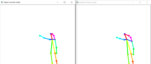
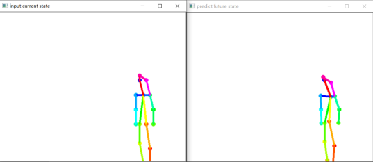
Therefore, today we will use torch to build LSTM to realize the real-time training and prediction of badminton action. In this paper, it is divided into several steps: data set production, data processing, model building and visualization. The effects of the model in 2000 rounds of training are as follows (the left side is the current action, and the right side is the predicted badminton action after the next 10 frames):

Introduction to the development of badminton movement recognition

For the recognition of badminton hitting action, Chu et al. Used the method based on pose recognition to extract the directional gradient histogram HOG from the player's boundary box, and classified the hitting action based on the HOG based on support vector machine SVM, but the training and test data used are a single image at the moment of hitting the ball, For different strokes with very similar hitting posture, it is likely to be confused, such as killing and high-distance ball, flat draw and hanging ball. Careelmont classifies the shot of compressed badminton video, and recognizes the hitting action by detecting the moving track of badminton. Ramasinghe et al. Proposed a badminton video action recognition method based on HOG feature of dense trajectory and trajectory alignment. Players' hitting actions are divided into forehand hitting, backhand hitting, killing and other types, but HOG itself does not have scale invariance, and HOG is quite sensitive to noise due to the nature of gradient. Under the background that sports video often has poor pixel quality and low resolution of non static video and image, Yang Jing and others proposed a motion descriptor based on optical flow, and captured the player's swing image by detecting key audio elements. Finally, support vector machine was used to analyze the three typical swing movements of athletes - up swing, left swing Right swing for classification. Wang et al. Proposed a double-layer hidden Markov model classification algorithm based on body sensor network to identify badminton hitting types, but it is not suitable for effective recognition of badminton actions in video for the hitting state data captured by sensors. Rahmad et al. Compared the performance of four different deep convolution pre training models, Alex net, GoogLeNet, VggNet-16 and VggNet-19, in classifying badminton game images to identify different actions of athletes. Finally, it showed that GoogLeNet had the highest classification accuracy, but it was still aimed at the static image of the moment of hitting the ball in badminton game, Failed to classify and recognize the badminton action meta video.

Badminton movement prediction

In order to better study the badminton video action recognition, we realize the time-domain positioning of badminton video players' hitting action.

Here, the program design is divided into the following steps: data set making, data processing, model building and visualization.

2.1 bone dataset extraction

Here we put the prepared video material under the project file and use data_deal.py extract bone point storage. For 2 Mp4 video file uses openpose to extract bone data frame by frame and store it in txt file. The code is as follows:

parser = argparse.ArgumentParser(description='Action Recognition by OpenPose')
parser.add_argument('--video', help='Path to video file.')
args = parser.parse_args()
# Import related models
estimator = load_pretrain_model('VGG_origin')
# Parameter initialization
realtime_fps = '0.0000'
start_time = time.time()
fps_interval = 1
fps_count = 0
run_timer = 0
frame_count = 0
# Read and write video files
cap =cv.VideoCapture("2.mp4")
#video_writer = set_video_writer(cap, write_fps=int(7.0))
# Save the txt file of joint data for training
f = open('origin_data.txt', 'a+')
num=0
while cv.waitKey(1) < 0:
    has_frame, show = cap.read()
    if has_frame:
        fps_count += 1
        frame_count += 1
        # pose estimation
        humans = estimator.inference(show)
        # get pose info
        pose = TfPoseVisualizer.draw_pose_rgb(show, humans)  # return frame, joints, bboxes, xcenter
        #video_writer.write(show)
        if len(pose[-1])==36:
            num+=1
            print(num)
            # Collect data for training
            joints_norm_per_frame = np.array(pose[-1]).astype(np.str)
            f.write(' '.join(joints_norm_per_frame))
            f.write('\n')
        cv.imshow("tets",show)
        cv.waitKey(1)
    else:
        break
cap.release()
f.close()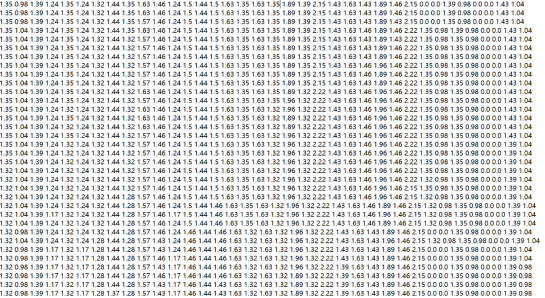

2.2 data processing

Through the observation of the data, it is found that because there are many occlusions in the captured video, the extraction of some limbs as 0 will greatly affect the model effect. These parts are removed here. The code is as follows:

f=open('origin_data.txt')
text=f.read()
f.close()
datasets=[]
text=text.split("\n")
for i in text:
    temp=i.split(" ")
    temp1=[]
    state=True
    for j in range(len(temp)):
        try:
            temp1.append(float(temp[j]))
        except:
            pass
    if len(temp1) == 36:
        temp1.pop(28)
        temp1.pop(28)
        temp1.pop(30)
        temp1.pop(30)
        for t in temp1:
            if t==0.:
                state=False
        if state:
            datasets.append(temp1)
flap=30#
x_data = datasets[:-1-flap]
y_data=datasets[flap:-1]
n=len(x_data)

2.3 LSTM model building and training

Here, the LSTM layer neuron 64 is set, the loss function is set as MSE error function, the optimizer is adam optimizer, the number of iterations is 100 rounds, and its loss diagram is drawn dynamically. The code is as follows:

times=[]
losss=[]
nums=0
Epoch=100
correct=0
for k in range(Epoch):
    for i in range(n):
        x_np=np.array(x_data[i],dtype='float32')#At this time, the dimension of x is 1
        y_np=np.array(y_data[i],dtype='float32')
        #The x dimension needs to be expanded to three dimensions, [batch,time_step,input_size]
        x=variable(torch.from_numpy(x_np[np.newaxis,:,np.newaxis]))
        y=variable(torch.from_numpy(y_np[np.newaxis,:,np.newaxis]))
        prediction=rnn(x)
        if prediction.flatten().data.numpy().any==y.flatten().data.numpy().any:
            correct+=1
        loss=loss_func(prediction,y)
        optim.zero_grad()
        loss.backward()
        optim.step()
        nums += 1
        accuracy=float(correct/nums)
print("|Epoch:",k,"|step:",nums,"|loss:",loss.data.numpy(),"|accuracy:%.4f"%accuracy)
        times.append(nums)
        losss.append(float(loss.data))
        plt.plot(times,losss)
        plt.pause(0.05)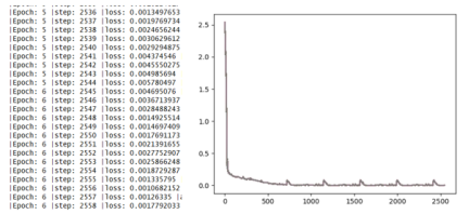

2.4 model visualization

According to the predicted bone coordinates, define the basic bone connection method and color. At the same time, consider the removed bones. The final code is as follows:

import cv2
def draw(test):
    back=cv2.imread("back.jpg")
    image_h, image_w ,c= back.shape
    centers = {}
    CocoColors = [[255, 0, 0], [255, 85, 0], [255, 170, 0], [255, 255, 0], [170, 255, 0], [85, 255, 0], [0, 255, 0],
                  [0, 255, 85], [0, 255, 170], [0, 255, 255], [0, 170, 255], [0, 85, 255], [0, 0, 255], [85, 0, 255],
                  [170, 0, 255], [255, 0, 255], [255, 0, 170], [255, 0, 85], [255, 0, 85]]
    CocoPairs = [
        (1, 2), (1, 5), (2, 3), (3, 4), (5, 6), (6, 7), (1, 8), (8, 9), (9, 10), (1, 11),
        (11, 12), (12, 13), (1, 0), (0, 14), (14, 15),  (5, 15)
    ]#Modified
    for pos in range(0,16):
        center = (int((test[2*pos] * (image_w//2) + 0.5)), int((test[2*pos+1] * (image_h//2) )))
        centers[pos] = center
        cv2.circle(back, center, 3, CocoColors[pos], thickness=3, lineType=8, shift=0)
    for pair_order, pair in enumerate(CocoPairs):
        cv2.line(back, centers[pair[0]], centers[pair[1]], CocoColors[pair_order], 3)

Full code:

https://download.csdn.net/download/qq_42279468/72398200

Li Qiujian, CSDN blog expert and author of CSDN talent course. Master is studying in China University of mining and technology, and has won prizes in taptap competition.