catalogue
First, Simulated annealing algorithm (SA).
2.SA solves the maximum value of the function
2.GA solves the maximum value of function
3, Particle swarm optimization (PSO)
4. Particle swarm optimization function
5. Advanced application of PSO algorithm
(2) Multivariate function fitting
(3) Fitting differential equation
First, Simulated annealing algorithm (SA).
1. Basic theory of SA
2.SA solves the maximum value of the function
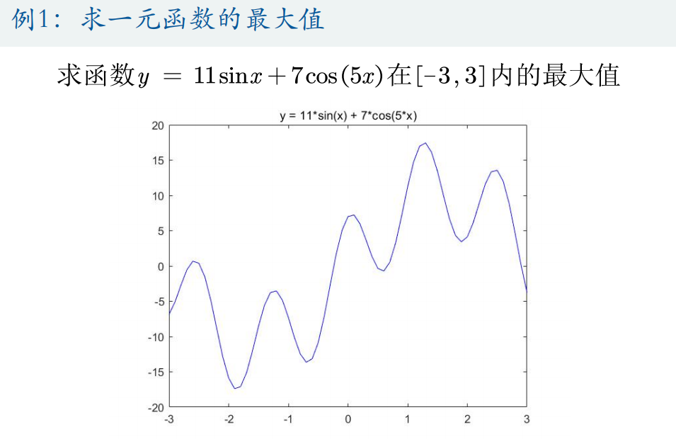
(1) Solve the maximum value of function y = 11*sin(x) + 7*cos(5*x) within [- 3,3]
%% Draw the graph of the function
x = -3:0.1:3;
y = 11*sin(x) + 7*cos(5*x);
figure
plot(x,y,'b-')
hold on
%% Parameter initialization
narvs = 1; % Number of variables
T0 = 100;   % initial temperature
T = T0; % The temperature will change during the iteration, and the temperature is zero at the first iteration T0
maxgen = 200;  % Maximum number of iterations
Lk = 100;  % Number of iterations per temperature
alfa = 0.95;  % Temperature attenuation coefficient
x_lb = -3; % x Lower bound of
x_ub = 3; % x Upper bound of

%%  Randomly generate an initial solution
x0 = zeros(1,narvs);
for i = 1: narvs
    x0(i) = x_lb(i) + (x_ub(i)-x_lb(i))*rand(1);
end
y0 = Obj_fun1(x0); % Calculate the function value of the current solution
h = scatter(x0,y0,'*r');  % scatter Is a function for drawing a two-dimensional scatter diagram (returned here) h In order to get the handle of the graph, we will update its position in the future)

%% Define some quantities to save the intermediate process, so as to facilitate the output of results and drawing
max_y = y0;     % The function value corresponding to the best solution found by initialization is y0
MAXY = zeros(maxgen,1); % Record the results found at the end of each outer cycle max_y ((convenient for drawing)

%% Simulated annealing process
for iter = 1 : maxgen  % External circulation, What I use here is to specify the maximum number of iterations
    for i = 1 : Lk  % Internal circulation, starting iteration at each temperature
        y = randn(1,narvs);  % Generate 1 line narvs Column N(0,1)random number
        z = y / sqrt(sum(y.^2)); % Calculate according to the generation rules of the new solution z
        x_new = x0 + z*T; % Calculate according to the generation rules of the new solution x_new Value of
        % If the position of the new solution exceeds the definition field, adjust it
        for j = 1: narvs
            if x_new(j) < x_lb(j)
                r = rand(1);
                x_new(j) = r*x_lb(j)+(1-r)*x0(j);
            elseif x_new(j) > x_ub(j)
                r = rand(1);
                x_new(j) = r*x_ub(j)+(1-r)*x0(j);
            end
        end
        x1 = x_new;    % The adjusted x_new Assign to new solution x1
        y1 = Obj_fun1(x1);  % Calculate the function value of the new solution
        if y1 > y0    % If the function value of the new solution is greater than the function value of the current solution
            x0 = x1; % Update current solution to new solution
            y0 = y1;
        else
            p = exp(-(y0 - y1)/T); % according to Metropolis The criterion calculates a probability
            if rand(1) < p   % Generate a random number and compare it with this probability. If the random number is less than this probability
                x0 = x1; % Update current solution to new solution
                y0 = y1;
            end
        end
        % Determine whether to update the best solution found
        if y0 > max_y  % If the current solution is better, update it
            max_y = y0;  % Update maximum y
            best_x = x0;  % Update the best found x
        end
    end
    MAXY(iter) = max_y; % Save the maximum value found after the end of this round of external circulation y
    T = alfa*T;   % Temperature drop
    pause(0.01)  % Pause for a period of time(Unit: Second)Then draw the picture
    h.XData = x0;  % Update the handle of the scatter chart x Axis data (at this time, the position of the solution changes on the diagram)
    h.YData = Obj_fun1(x0); % Update the handle of the scatter chart y Axis data (at this time, the position of the solution changes on the diagram)
end

disp('The best location is:'); disp(best_x)
disp('At this time, the optimal value is:'); disp(max_y)

pause(0.5)
h.XData = [];  h.YData = [];  % Delete the original scatter
scatter(best_x,max_y,'*r');  % Re mark the scatter at the maximum
title(['The maximum value found by simulated annealing is', num2str(max_y)])  % Add the title above

%% Draw the maximum value found after each iteration y Graphics of
figure
plot(1:maxgen,MAXY,'b-');
xlabel('Number of iterations');
ylabel('y Value of');
(2) Solve the minimum value of function y = x1^2+x2^2-x1*x2-10*x1-4*x2+60 in [- 15,15]
%% Draw the graph of the function
figure
x1 = -15:1:15;
x2 = -15:1:15;
[x1,x2] = meshgrid(x1,x2);
y = x1.^2 + x2.^2 - x1.*x2 - 10*x1 - 4*x2 + 60;
mesh(x1,x2,y)
xlabel('x1');  ylabel('x2');  zlabel('y');  % Label the axis
axis vis3d % Freeze the screen aspect ratio so that the rotation of a 3D object will not change the scale display of the coordinate axis
hold on
%% Parameter initialization
narvs = 2; % Number of variables
T0 = 100; % initial temperature
T = T0; % The temperature will change during the iteration, and the temperature is zero at the first iteration T0
maxgen = 200; % Maximum number of iterations
Lk = 100; % Number of iterations per temperature
alfa = 0.95; % Temperature attenuation coefficient
x_lb = [-15 -15]; % x Lower bound of
x_ub = [15 15]; % x Upper bound of
%% Randomly generate an initial solution
x0 = zeros(1,narvs);
for i = 1: narvs
x0(i) = x_lb(i) + (x_ub(i)-x_lb(i))*rand(1);
end
y0 = Obj_fun2(x0); % Calculate the function value of the current solution
h = scatter3(x0(1),x0(2),y0,'*r'); % scatter3 Is a function for drawing a three-dimensional scatter chart (returned here) h In order to get the handle of the graph, we will update its position in the future)
%% Define some quantities to save the intermediate process, so as to facilitate the output of results and drawing
min_y = y0; % The function value corresponding to the best solution found by initialization is y0
MINY = zeros(maxgen,1); % Record the results found at the end of each outer cycle min_y ((convenient for drawing)
%% Simulated annealing process
for iter = 1 : maxgen % External circulation, What I use here is to specify the maximum number of iterations
for i = 1 : Lk % Internal circulation, starting iteration at each temperature
y = randn(1,narvs); % Generate 1 line narvs Column N(0,1)random number
z = y / sqrt(sum(y.^2)); % Calculate according to the generation rules of the new solution z
x_new = x0 + z*T; % Calculate according to the generation rules of the new solution x_new Value of
% If the position of the new solution exceeds the definition field, adjust it
for j = 1: narvs
if x_new(j) < x_lb(j)
r = rand(1);
x_new(j) = r*x_lb(j)+(1-r)*x0(j);
elseif x_new(j) > x_ub(j)
r = rand(1);
x_new(j) = r*x_ub(j)+(1-r)*x0(j);
end
end
x1 = x_new; % The adjusted x_new Assign to new solution x1
y1 = Obj_fun2(x1); % Calculate the function value of the new solution
if y1 < y0 % If the function value of the new solution is less than the function value of the current solution
x0 = x1; % Update current solution to new solution
y0 = y1;
else
p = exp(-(y1 - y0)/T); % according to Metropolis The criterion calculates a probability
if rand(1) < p % Generate a random number and compare it with this probability. If the random number is less than this probability
x0 = x1; % Update current solution to new solution
y0 = y1;
end
end
% Determine whether to update the best solution found
if y0 < min_y % If the current solution is better, update it
min_y = y0; % Update minimum y
best_x = x0; % Find the best update x
end
end
MINY(iter) = min_y; % Save the smallest found after the end of this round of external circulation y
T = alfa*T; % Temperature drop
pause(0.02) % After a pause(Unit: Second)Then draw the picture
h.XData = x0(1); % Update the handle of the scatter chart x Axis data (at this time, the position of the solution changes on the diagram)
h.YData = x0(2); % Update the handle of the scatter chart y Axis data (at this time, the position of the solution changes on the diagram)
h.ZData = Obj_fun2(x0); % Update the handle of the scatter chart z Axis data (at this time, the position of particles changes on the graph)
end
disp('The best location is:'); disp(best_x)
disp('At this time, the optimal value is:'); disp(min_y)
pause(0.5)
h.XData = []; h.YData = []; h.ZData = []; % Delete the original scatter
scatter3(best_x(1), best_x(2), min_y,'*r'); % Re mark the scatter at the minimum value
title(['The minimum value found by simulated annealing is', num2str(min_y)]) % Add the title above
%% Draw the minimum number found after each iteration y Graphics of
figure
plot(1:maxgen,MINY,'b-');
xlabel('Number of iterations');
ylabel('y Value of');(3) TSP problem
tic
rng('shuffle') % Control the generation of random numbers, otherwise it is opened every time matlab The results are the same
% https://ww2.mathworks.cn/help/matlab/math/why-do-random-numbers-repeat-after-startup.html
% https://ww2.mathworks.cn/help/matlab/ref/rng.html
clear;clc
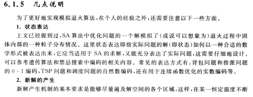
% 38 A city, TSP Dataset website(http://www.tsp. gatech. edu/world/djtour. The best result of public test on HTML is 6656.
coord = [11003.611100,42102.500000;11108.611100,42373.888900;11133.333300,42885.833300;11155.833300,42712.500000;11183.333300,42933.333300;11297.500000,42853.333300;11310.277800,42929.444400;11416.666700,42983.333300;11423.888900,43000.277800;11438.333300,42057.222200;11461.111100,43252.777800;11485.555600,43187.222200;11503.055600,42855.277800;11511.388900,42106.388900;11522.222200,42841.944400;11569.444400,43136.666700;11583.333300,43150.000000;11595.000000,43148.055600;11600.000000,43150.000000;11690.555600,42686.666700;11715.833300,41836.111100;11751.111100,42814.444400;11770.277800,42651.944400;11785.277800,42884.444400;11822.777800,42673.611100;11846.944400,42660.555600;11963.055600,43290.555600;11973.055600,43026.111100;12058.333300,42195.555600;12149.444400,42477.500000;12286.944400,43355.555600;12300.000000,42433.333300;12355.833300,43156.388900;12363.333300,43189.166700;12372.777800,42711.388900;12386.666700,43334.722200;12421.666700,42895.555600;12645.000000,42973.333300];
n = size(coord,1); % Number of cities
figure % Create a new graphic window
plot(coord(:,1),coord(:,2),'o'); % Draw a scatter diagram of the distribution of the city
hold on % Wait a minute. I'm going to draw on this figure
d = zeros(n); % Initialize the distance matrix of two cities to 0
for i = 2:n
for j = 1:i
coord_i = coord(i,:); x_i = coord_i(1); y_i = coord_i(2); % city i The abscissa of is x_i,The ordinate is y_i
coord_j = coord(j,:); x_j = coord_j(1); y_j = coord_j(2); % city j The abscissa of is x_j,The ordinate is y_j
d(i,j) = sqrt((x_i-x_j)^2 + (y_i-y_j)^2); % Computing City i and j Distance
end
end
d = d+d'; % Generate the symmetrical side of the distance matrix
%% Parameter initialization
T0 = 1000; % initial temperature
T = T0; % The temperature will change during the iteration. The temperature is zero at the first iteration T0
maxgen = 1000; % Maximum number of iterations
Lk = 500; % Number of iterations per temperature
alpfa = 0.95; % Temperature attenuation coefficient
%% Randomly generate an initial solution
path0 = randperm(n); % Generate a 1-n As a random sequence of initial paths
result0 = calculate_tsp_d(path0,d); % Call what we wrote ourselves calculate_tsp_d Function to calculate the distance of the current path
%% Define some quantities to save the intermediate process, so as to facilitate the output of results and drawing
min_result = result0; % The distance corresponding to the best solution found by initialization is result0
RESULT = zeros(maxgen,1); % Record the results found at the end of each outer cycle min_result ((convenient for drawing)
%% Simulated annealing process
for iter = 1 : maxgen % External circulation, What I use here is to specify the maximum number of iterations
for i = 1 : Lk % Internal circulation, starting iteration at each temperature
path1 = gen_new_path(path0); % Call what we wrote ourselves gen_new_path Function to generate a new path
result1 = calculate_tsp_d(path1,d); % Calculate the distance of the new path
%If the distance of the new solution is short, the value of the new solution is directly assigned to the original solution
if result1 < result0
path0 = path1; % Update current path to new path
result0 = result1;
else
p = exp(-(result1 - result0)/T); % according to Metropolis The criterion calculates a probability
if rand(1) < p % Generate a random number and compare it with this probability. If the random number is less than this probability
path0 = path1; % Update current path to new path
result0 = result1;
end
end
% Determine whether to update the best solution found
if result0 < min_result % If the current solution is better, update it
min_result = result0; % Update minimum distance
best_path = path0; % Update the shortest path found
end
end
RESULT(iter) = min_result; % Save the minimum distance found after the end of this round of external circulation
T = alpfa*T; % Temperature drop
end
disp('The best solution is:'); disp(mat2str(best_path))
disp('At this time, the optimal value is:'); disp(min_result)
best_path = [best_path,best_path(1)]; % Add an element on the last side of the shortest path, that is, the first point (we want to generate a closed graph)
n = n+1; % Number of cities plus one (following the previous step)
for i = 1:n-1
j = i+1;
coord_i = coord(best_path(i),:); x_i = coord_i(1); y_i = coord_i(2);
coord_j = coord(best_path(j),:); x_j = coord_j(1); y_j = coord_j(2);
plot([x_i,x_j],[y_i,y_j],'-b') % Make a line segment at every two points until all the cities are finished
% pause(0.02) % Pause 0.02s Draw the next line segment
hold on
end
%% Draw the graph of the shortest path found after each iteration
figure
plot(1:maxgen,RESULT,'b-');
xlabel('Number of iterations');
ylabel('Shortest path');
toc
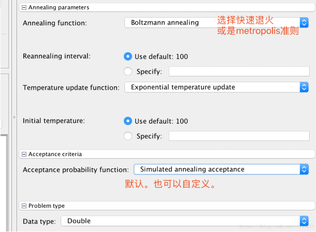
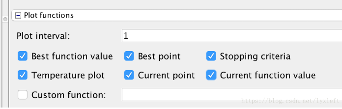
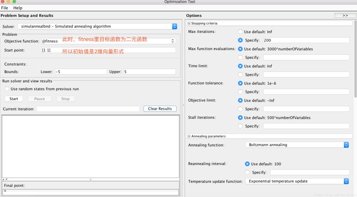
3.SA toolbox
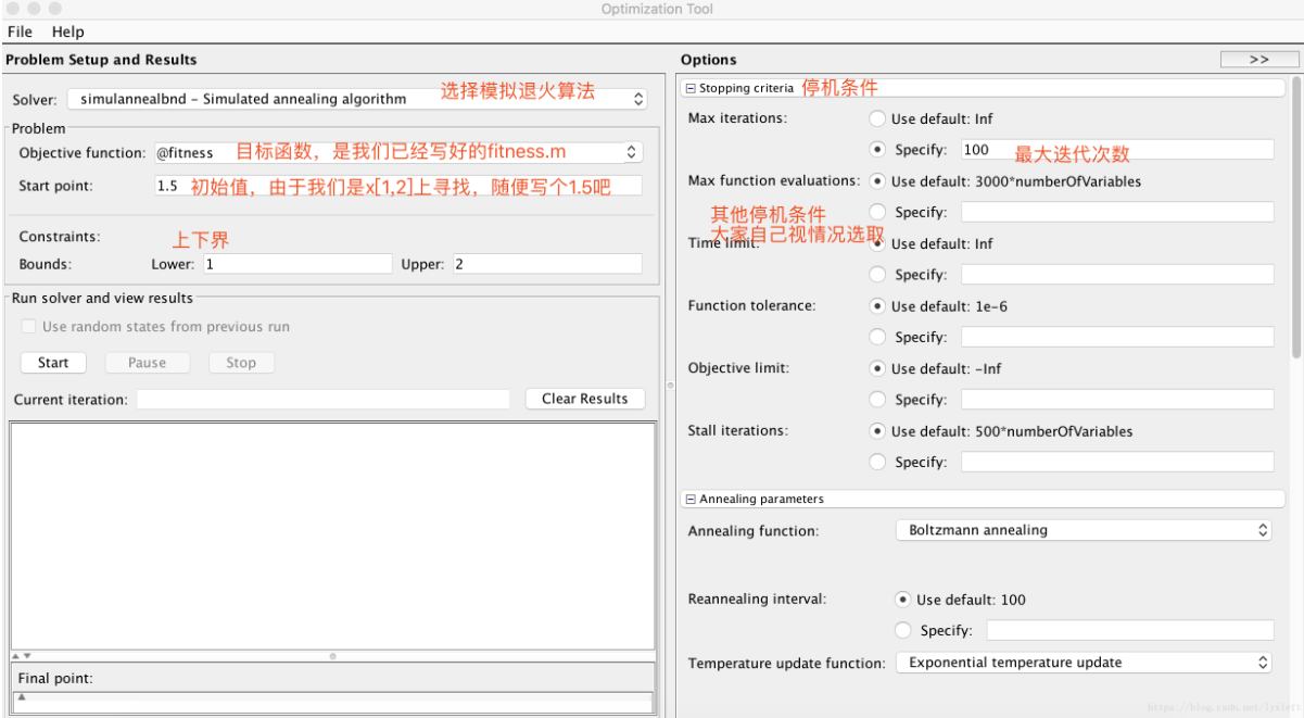
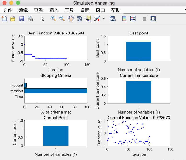
(1) Solve the extreme value of univariate function: y = sin(10*pi*x) / x in the range of x = [1,2]
<fitness.m>
function fitnessVal = fitness( x )

% Univariate function optimization:

fitnessVal = sin(10*pi*x) / x;  %Find the minimum value

% fitnessVal = -1 * sin(10*pi*x) / x; Using simulated annealing to find the maximum value, you can add a minus sign or make a reciprocal!

end
(2) Solve the binary function: find the extreme value of z = x.^2 + y.^2 - 10*cos(2*pi*x) - 10*cos(2*pi*y) + 20 in the range where x and y are [- 5,5]
<fitness.m>
function fitnessVal = fitness( x )

% Binary function optimization:

fitnessVal = -1 * (x(1)^2 + x(2).^2 - 10*cos(2*pi*x(1)) - 10*cos(2*pi*x(2)) + 20);

end
2, Genetic algorithm (GA)
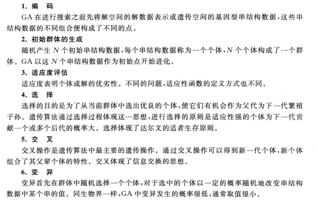
1. Theoretical basis of GA
2.GA solves the maximum value of function
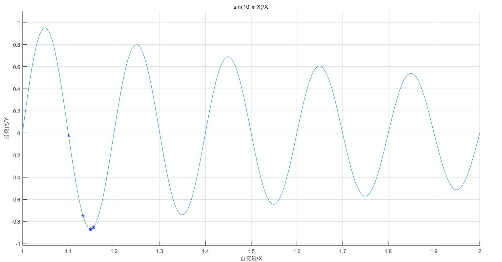
(1) Solve the unary function: the minimum value of sin(10*pi*X)/X in the range of [1,2]
clc
clear all
close all
%% Draw a function diagram
figure(1);
hold on;
lb=1;ub=2; %Function argument range [1],2]
ezplot('sin(10*pi*X)/X',[lb,ub]); %Draw the function curve
xlabel('independent variable/X')
ylabel('function value/Y')
%% Defining genetic algorithm parameters
NIND=40; %Number of individuals
MAXGEN=20; %Maximum genetic algebra
PRECI=20; %Precision of variables
GGAP=0.95; %generation gap
px=0.7; %Crossover probability
pm=0.01; %Variation probability
trace=zeros(2,MAXGEN); %Initial value of optimization result
FieldD=[PRECI;lb;ub;1;0;1;1]; %Area descriptor
Chrom=crtbp(NIND,PRECI); %Initial population
%% optimization
gen=0; %Generation counter
X=bs2rv(Chrom,FieldD); %Calculate the decimal conversion of the initial population
ObjV=sin(10*pi*X)./X; %Calculate the objective function value
while gen<MAXGEN
FitnV=ranking(ObjV); %Assign fitness values
SelCh=select('sus',Chrom,FitnV,GGAP); %choice
SelCh=recombin('xovsp',SelCh,px); %recombination
SelCh=mut(SelCh,pm); %variation
X=bs2rv(SelCh,FieldD); %Decimal conversion of descendant individuals
ObjVSel=sin(10*pi*X)./X; %Calculate the objective function value of offspring
[Chrom,ObjV]=reins(Chrom,SelCh,1,1,ObjV,ObjVSel); %Reintroduce the offspring to the parent to obtain a new population
X=bs2rv(Chrom,FieldD);
gen=gen+1; %Generation counter increase
%Obtain the optimal solution of each generation and its serial number, Y Is the optimal solution,I Is the serial number of the individual
[Y,I]=min(ObjV);
trace(1,gen)=X(I); %Note the optimal value of each generation
trace(2,gen)=Y; %Note the optimal value of each generation
end
plot(trace(1,:),trace(2,:),'bo'); %Draw the best of each generation
grid on;
plot(X,ObjV,'b*'); %Draw the last generation of the population
hold off
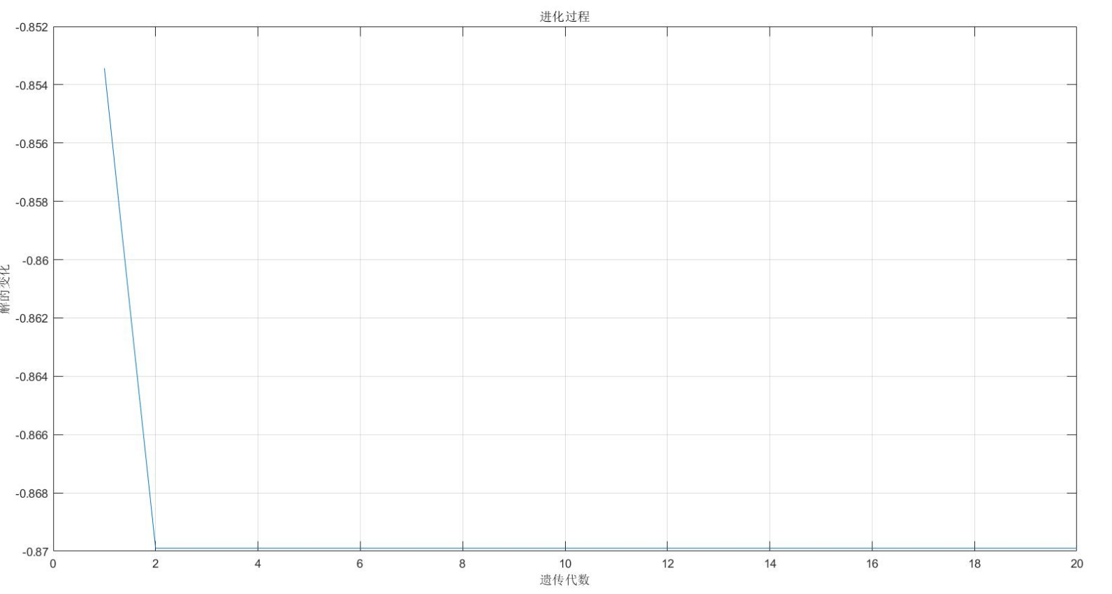
%% Draw an evolution map
figure(2);
plot(1:MAXGEN,trace(2,:));
grid on
xlabel('Genetic algebra')
ylabel('Change of solution')
title('evolutionary process ')
bestY=trace(2,end);
bestX=trace(1,end);
fprintf(['Optimal solution:\nX=',num2str(bestX),'\nY=',num2str(bestY),'\n'])
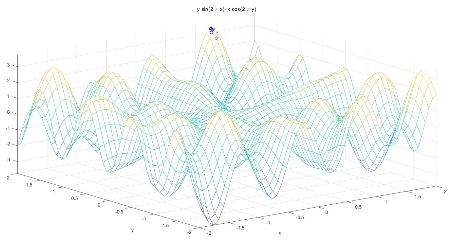
(2) Solve the binary function: X and y are in the range of [- 2,2], and the maximum value of y*sin(2*pi*x)+x*cos(2*pi*y)
clc
clear all
close all
%% Draw a function diagram
figure(1);
lbx=-2;ubx=2; %Function argument x Scope[-2,2]
lby=-2;uby=2; %Function argument y Scope[-2,2]
ezmesh('y*sin(2*pi*x)+x*cos(2*pi*y)',[lbx,ubx,lby,uby],50); %Draw the function curve
hold on;
%% Defining genetic algorithm parameters
NIND=40; %Number of individuals
MAXGEN=50; %Maximum genetic algebra
PRECI=20; %Precision of variables
GGAP=0.95; %generation gap
px=0.7; %Crossover probability
pm=0.01; %Variation probability
trace=zeros(3,MAXGEN); %Initial value of optimization result
FieldD=[PRECI PRECI;lbx lby;ubx uby;1 1;0 0;1 1;1 1]; %Area descriptor
Chrom=crtbp(NIND,PRECI*2); %Initial population
%% optimization
gen=0; %Generation counter
XY=bs2rv(Chrom,FieldD); %Calculate the decimal conversion of the initial population
X=XY(:,1);Y=XY(:,2);
ObjV=Y.*sin(2*pi*X)+X.*cos(2*pi*Y); %Calculate the objective function value
while gen<MAXGEN
FitnV=ranking(-ObjV); %Assign fitness values
SelCh=select('sus',Chrom,FitnV,GGAP); %choice
SelCh=recombin('xovsp',SelCh,px); %recombination
SelCh=mut(SelCh,pm); %variation
XY=bs2rv(SelCh,FieldD); %Decimal conversion of offspring individuals
X=XY(:,1);Y=XY(:,2);
ObjVSel=Y.*sin(2*pi*X)+X.*cos(2*pi*Y); %Calculate the objective function value of offspring
[Chrom,ObjV]=reins(Chrom,SelCh,1,1,ObjV,ObjVSel); %Reintroduce the offspring to the parent to obtain a new population
XY=bs2rv(Chrom,FieldD);
gen=gen+1; %Generation counter increase
%Obtain the optimal solution of each generation and its serial number, Y Is the optimal solution,I Is the serial number of the individual
[Y,I]=max(ObjV);
trace(1:2,gen)=XY(I,:); %Note the optimal value of each generation
trace(3,gen)=Y; %Note the optimal value of each generation
end
plot3(trace(1,:),trace(2,:),trace(3,:),'bo'); %Draw the best of each generation
grid on;
plot3(XY(:,1),XY(:,2),ObjV,'bo'); %Draw the last generation of the population
hold off
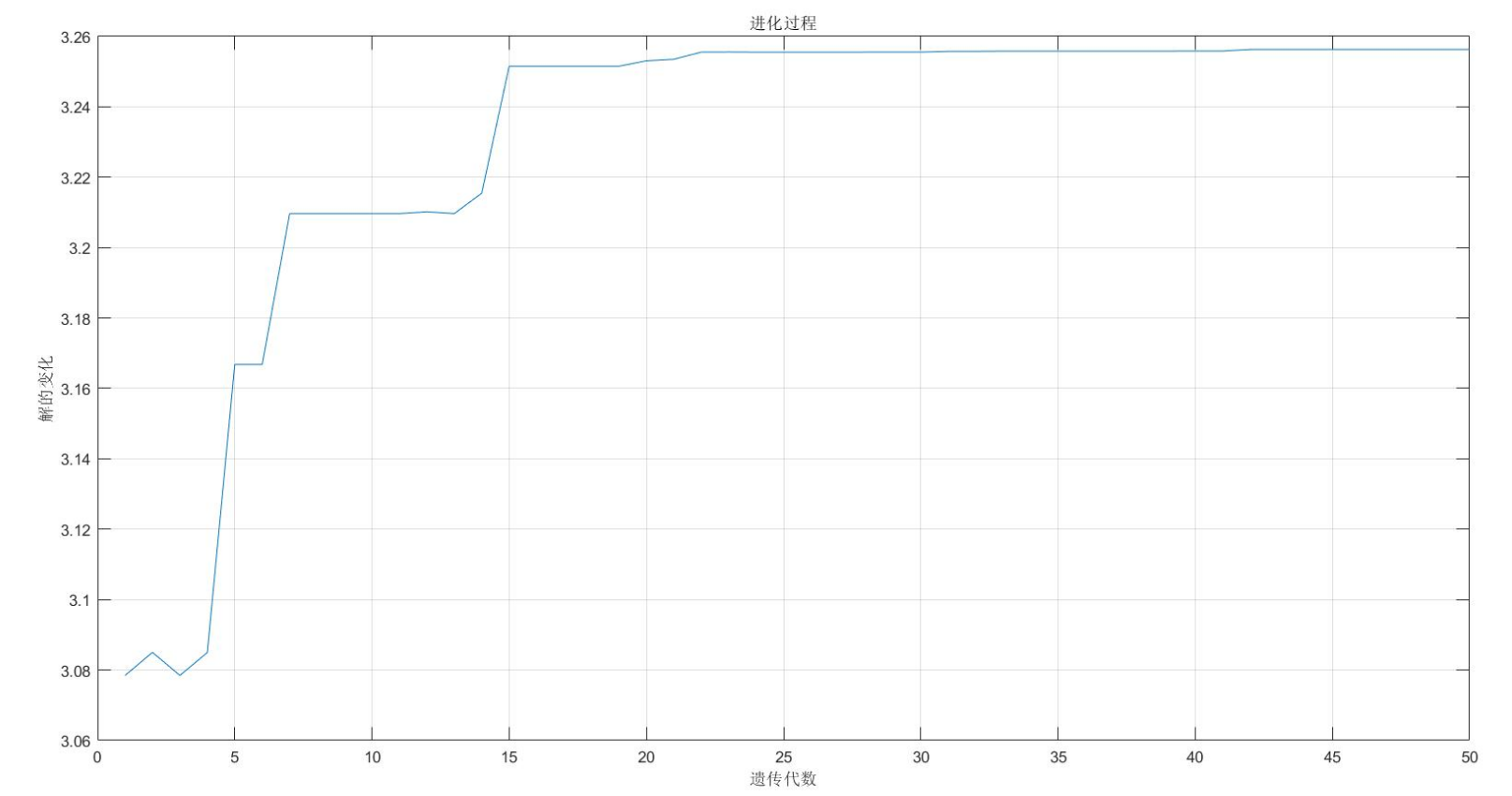
%% Draw an evolution map
figure(2);
plot(1:MAXGEN,trace(3,:));
grid on
xlabel('Genetic algebra')
ylabel('Change of solution')
title('evolutionary process ')
bestZ=trace(3,end);
bestX=trace(1,end);
bestY=trace(2,end);
fprintf(['Optimal solution:\nX=',num2str(bestX),'\nY=',num2str(bestY),'\nZ=',num2str(bestZ),'\n'])
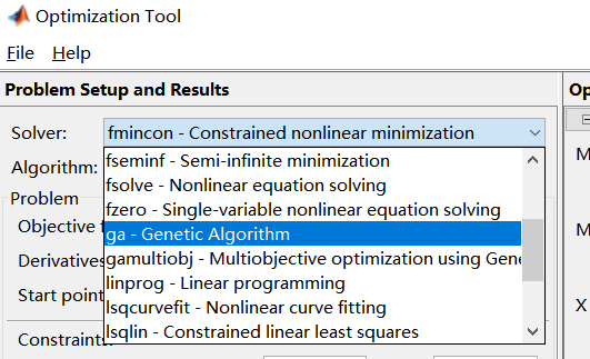
3.GA toolbox
Genetic algorithm is one of the modern optimization algorithms. It provides a genetic algorithm toolbox for easy use of Matlab, which can facilitate us to solve general optimization problems.

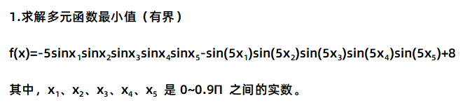
① preparation of objective function (fitness)
<fun.m>
function y=fun(x)
y=-5*sin(x(1))*sin(x(2))*sin(x(3))*sin(x(4))*sin(x(5))...
-sin(5*x(1))*sin(5*x(2))*sin(5*x(3))*sin(5*x(4))*sin(5*x(5))+8;
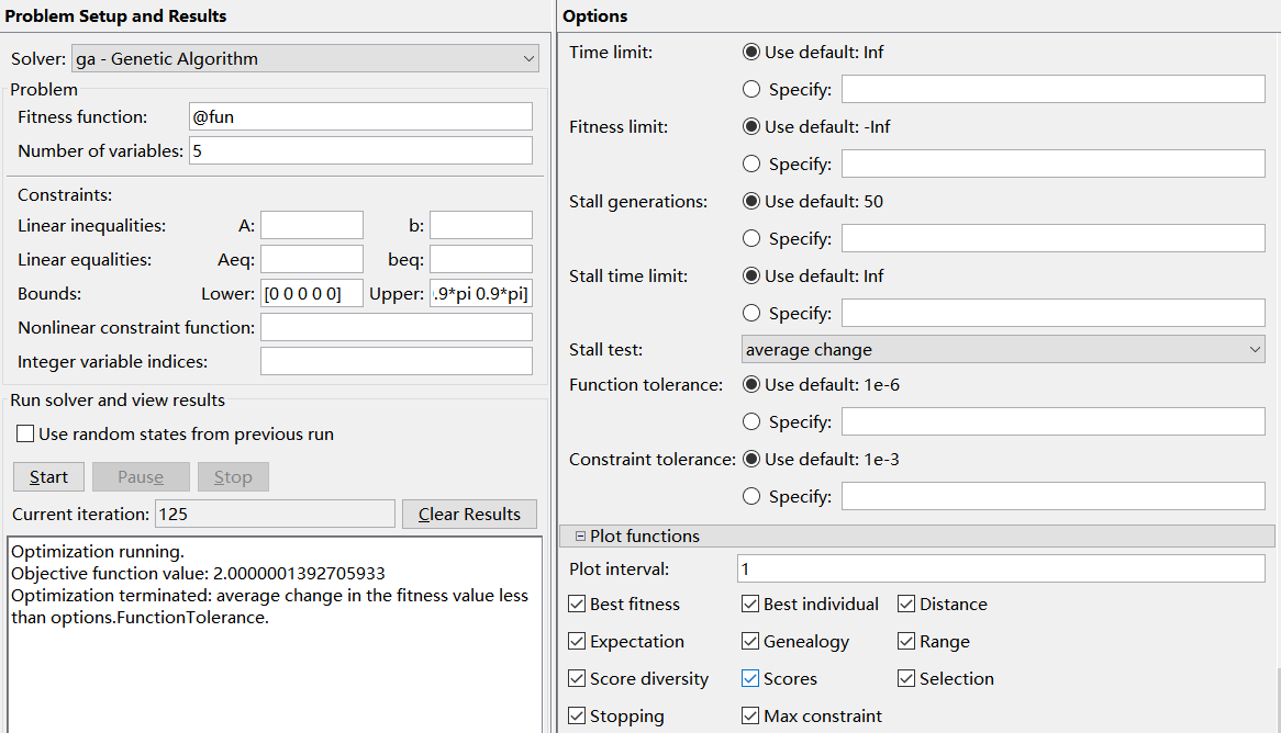
end② Input parameters
Enter @ target function name at Fitness function (because the function handle is passed here, so you must add @, otherwise an error will occur). Number of Variables refers to the Number of Variables to be solved. Next, enter the constraint condition, so that xi is a real number between 0 and 0.9pi, So you just need to enter at Bound, and then click the Start button to get the result.
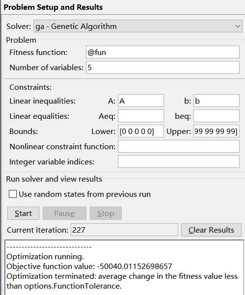
2. Solve the maximum value (bounded) of multivariate function with linear inequality constraints
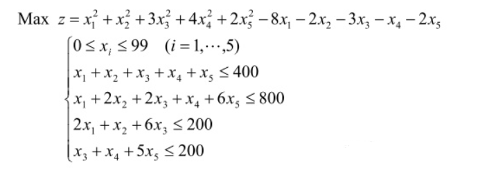
This is to find the maximum value, but the genetic algorithm toolbox can only find the minimum value, so when we write the fitness function, just add a negative sign in front of the objective function (when - z is the smallest, z is the largest).
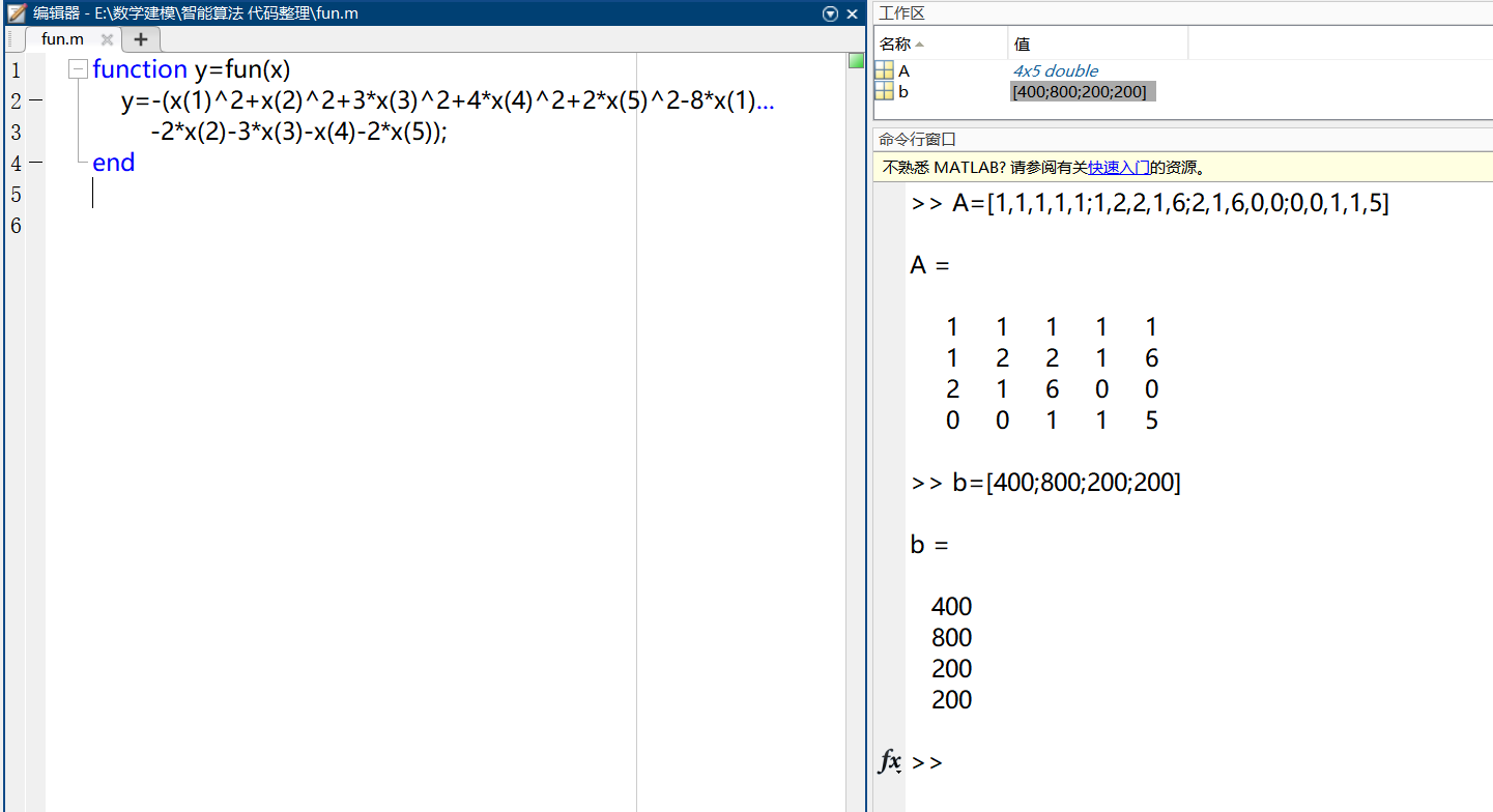
① write fitness function (objective function)
<fun.m>
function y=fun(x)
    y=-(x(1)^2+x(2)^2+3*x(3)^2+4*x(4)^2+2*x(5)^2-8*x(1)...
        -2*x(2)-3*x(3)-x(4)-2*x(5));
end
② Linear inequality constraints are defined in Matlab, and the expression of inequality constraints is:
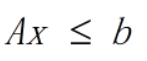
There should be matrix variables with constraints in the workspace. Unlike example 1, you only need to add inequality constraints at the constraints. This is the opposite of the maximum.
③ Input parameters
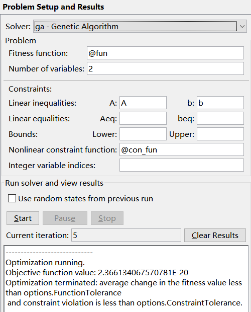
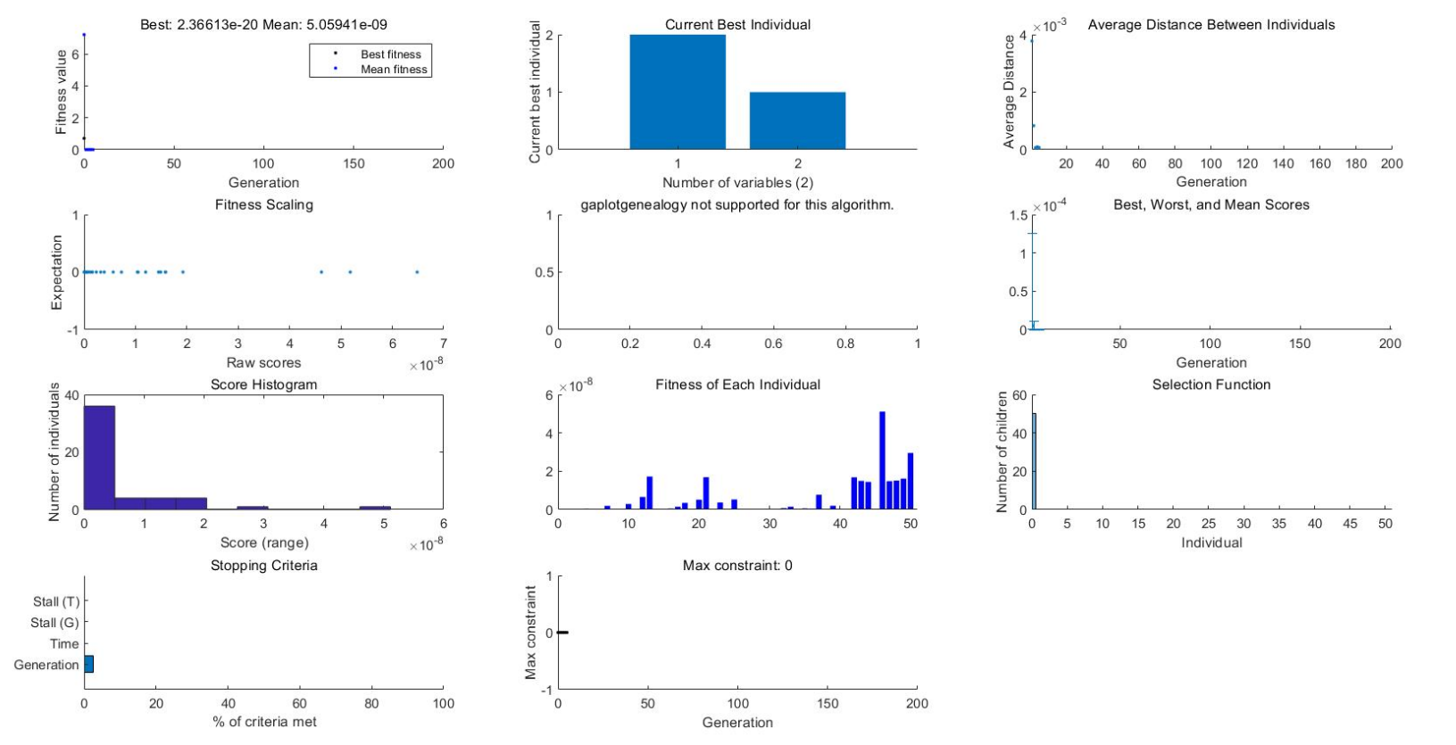
3. Solve the minimum value of multivariate function with nonlinear inequality constraints
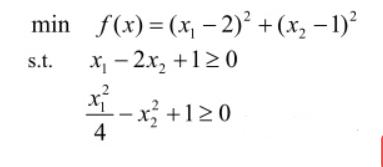
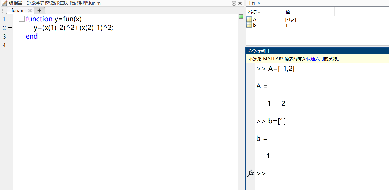
① write fitness function (objective function)
<fun.m>
function y=fun(x)
    y=(x(1)-2)^2+(x(2)-1)^2;
end
② Define linear inequality constraints
③ Write nonlinear inequality constraints
<con_fun.m>
function [c,ceq]=con_fun(x)
    c=-(1/4*x(1)^2-x(2)^2+1);
    ceq=[]
end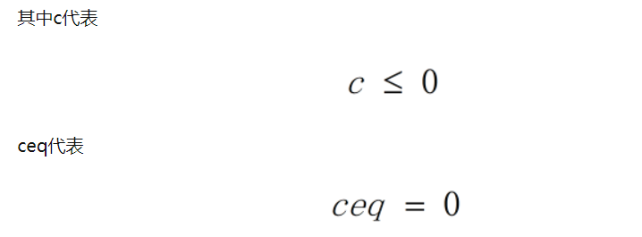
④ Input parameters
Compared with the previous question, you need to input the nonlinear constraint m file function in Constraints.
The parameters not involved in the above example are Aeq and beq, which are the conditions of linear equality constraints, and the parameters at Inter variable indexes (which indicates that the parameter is an integer). For details, see Quick Reference.
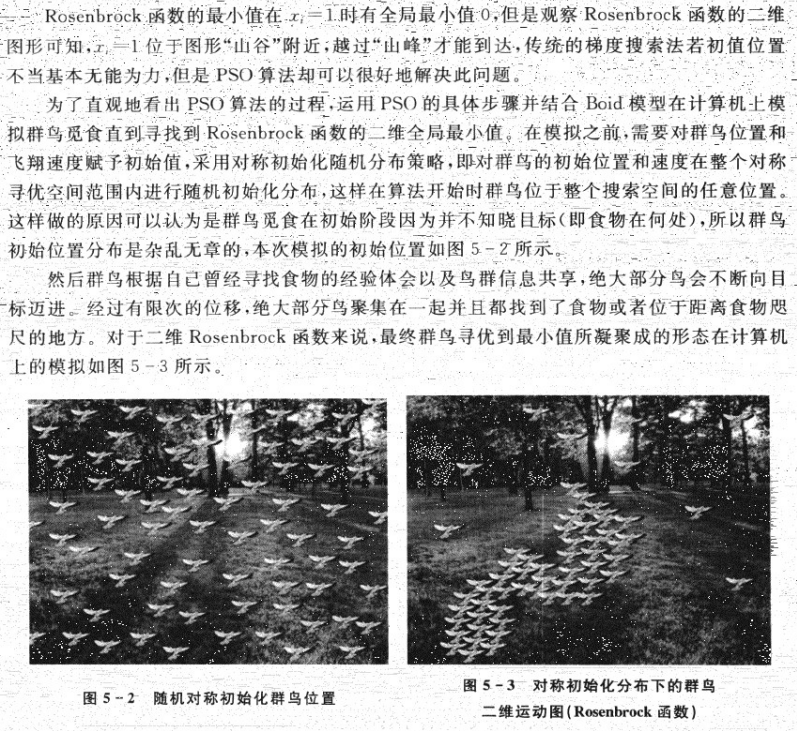
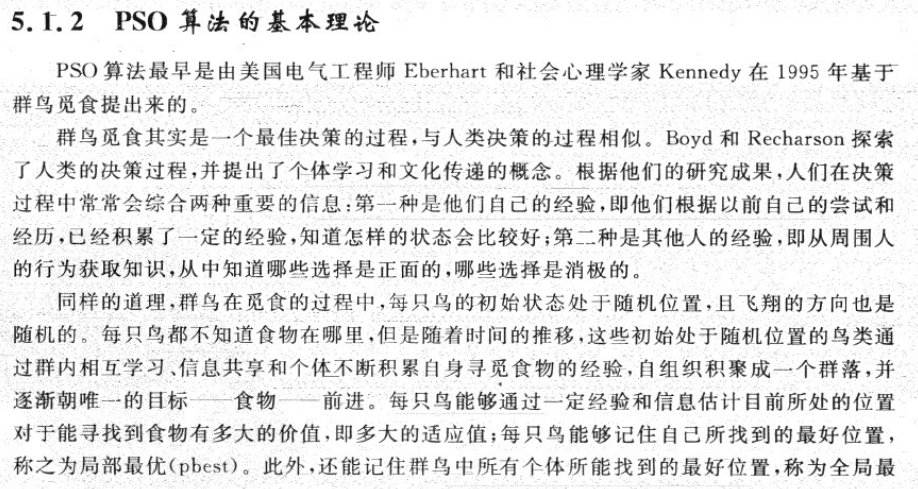
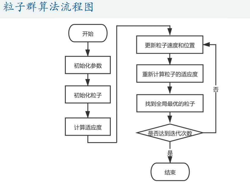
3, Particle swarm optimization (PSO)
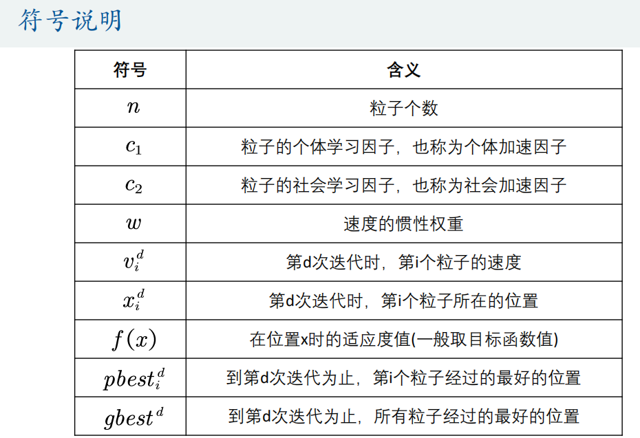
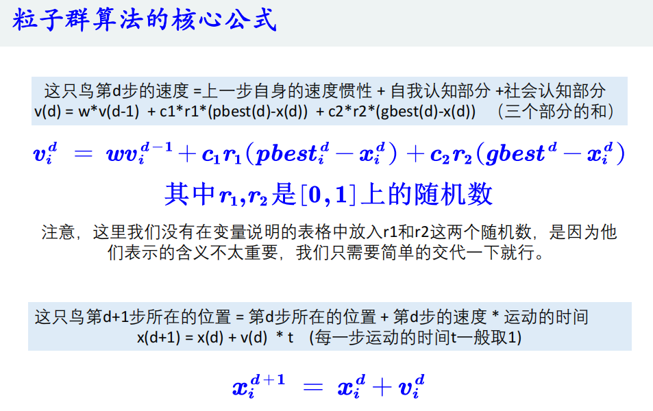
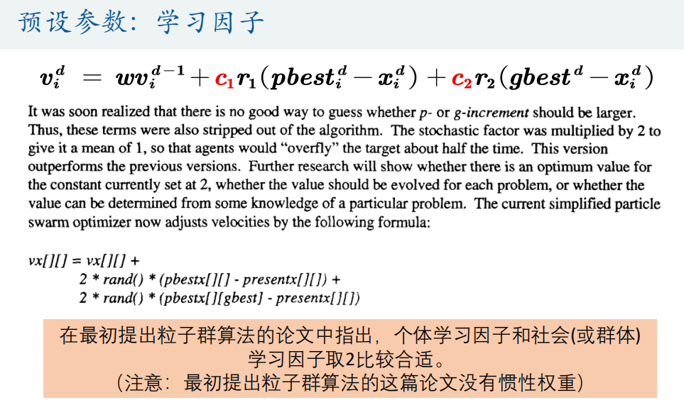
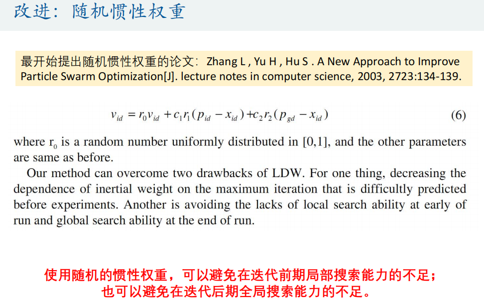
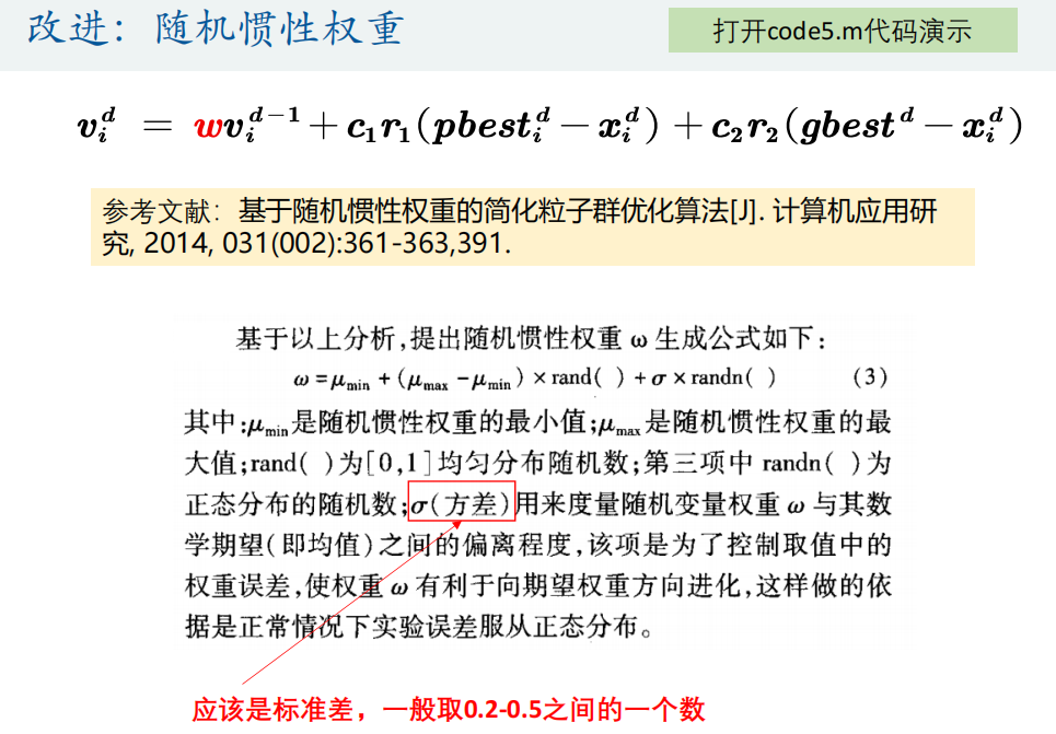
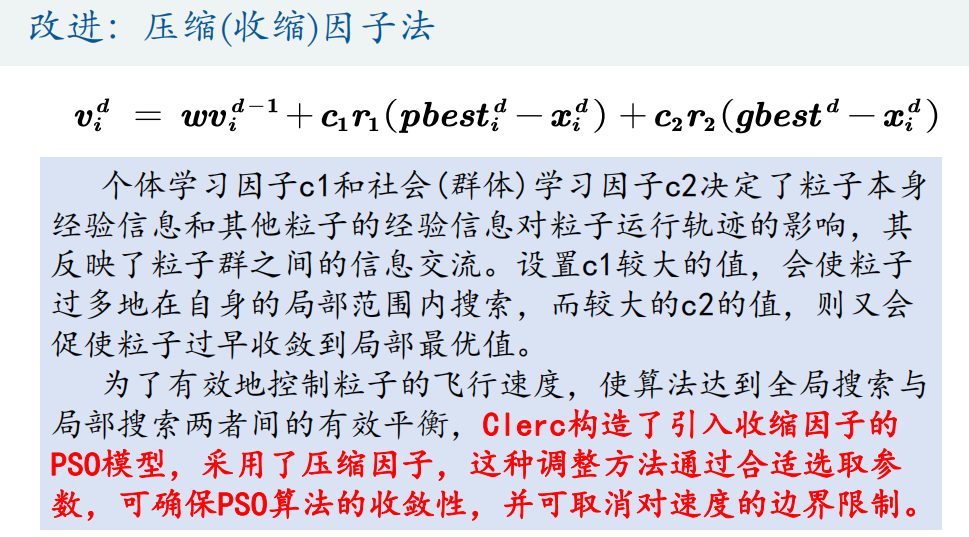
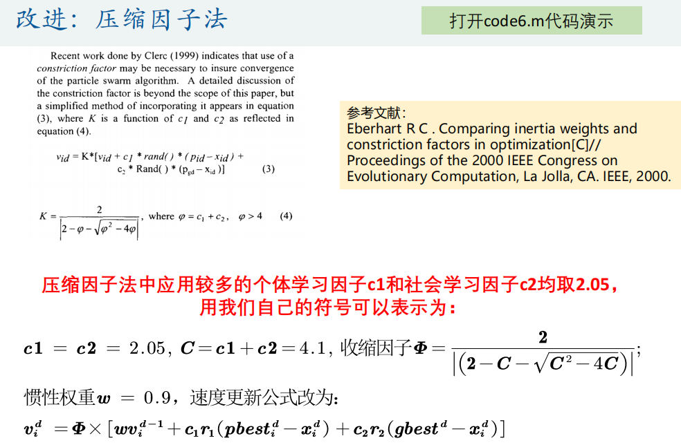
1. Knowledge of PSO algorithm

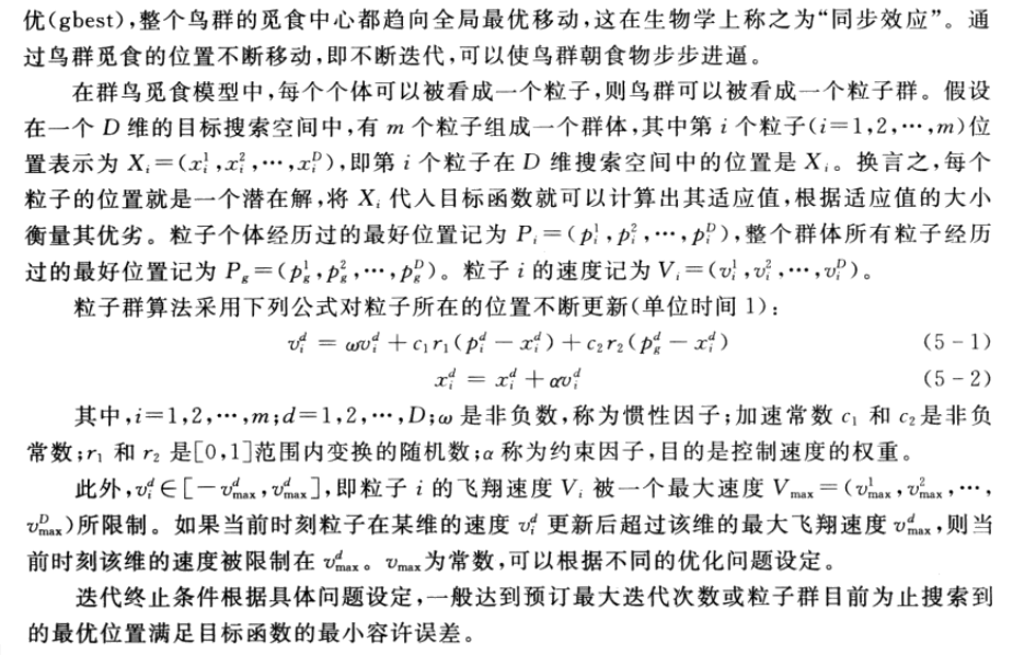
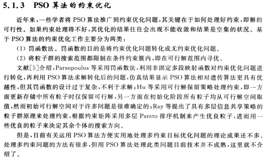

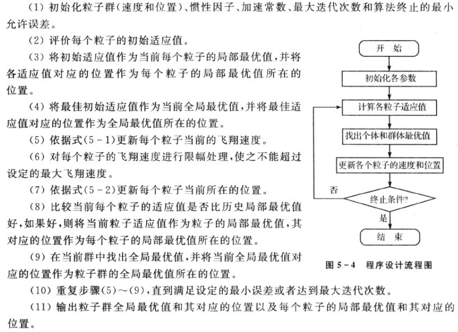
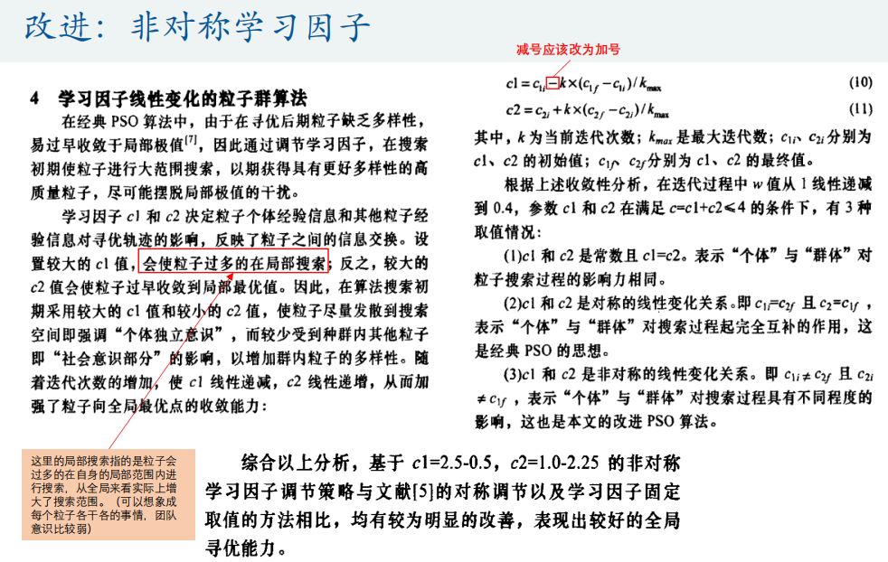
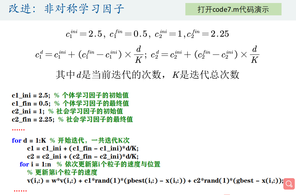
2.PSO algorithm design
3.PSO algorithm


Matlab code:
%% Draw the graph of the function
x = -3:0.01:3;
y = 11*sin(x) + 7*cos(5*x);
figure(1)
plot(x,y,'b-')
title('y = 11*sin(x) + 7*cos(5*x)')
hold on
%% The parameters in the particle swarm optimization algorithm can be modified instead of the preset parameters
n = 10; % Number of particles
narvs = 1; % Number of variables
c1 = 2; % The individual learning factor of each particle, also known as the individual acceleration constant
c2 = 2; % The social learning factor of each particle is also called social acceleration constant
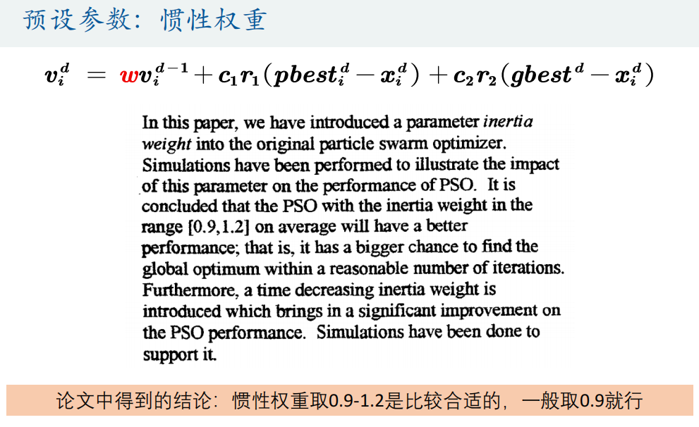
w = 0.9; % Inertia weight
K = 50; % Number of iterations
vmax = 1.2; % Maximum velocity of particles
x_lb = -3; % x Lower bound of
x_ub = 3; % x Upper bound of
%% Initializes the position and velocity of particles
x = zeros(n,narvs);
for i = 1: narvs
x(:,i) = x_lb(i) + (x_ub(i)-x_lb(i))*rand(n,1); % The position of the randomly initialized particle is within the definition domain
end
v = -vmax + 2*vmax .* rand(n,narvs); % The speed of randomly initialized particles (here we set it to[-vmax,vmax])
% Namely: v = -repmat(vmax, n, 1) + 2*repmat(vmax, n, 1) .* rand(n,narvs);
% be careful: x The initialization of can also be written in one line: x = x_lb + (x_ub-x_lb).*rand(n,narvs) ,Principle and v The calculation is the same
%% Calculate fitness
fit = zeros(n,1); % Initialize this n The fitness of all particles is 0
for i = 1:n % Cycle the whole particle swarm and calculate the fitness of each particle
fit(i) = Obj_fun1(x(i,:)); % call Obj_fun1 Function to calculate fitness (written here as x(i,:)Mainly for interworking with multivariate functions encountered later)
end
pbest = x; % Initialize this n The best position a particle has found so far n*narvs (vector of)
ind = find(fit == max(fit), 1); % Find the subscript of the particle with the greatest fitness
gbest = x(ind,:); % Defines the best position all particles have found so far (a 1*narvs (vector of)
%% Mark this on the picture n The position of particles is used for demonstration
h = scatter(x,fit,80,'*r'); % scatter Is a function of drawing a two-dimensional scatter diagram,80 Is the size of the scatter display I set (returned here) h In order to get the handle of the graph, we will update its position in the future)
%% iteration K To update the speed and position
fitnessbest = ones(K,1); % Initialize the best fitness obtained in each iteration
for d = 1:K % Start iteration, total iteration K second
for i = 1:n % Update page in sequence i Velocity and position of particles
v(i,:) = w*v(i,:) + c1*rand(1)*(pbest(i,:) - x(i,:)) + c2*rand(1)*(gbest - x(i,:)); % Update page i Velocity of particles
% If the particle's speed exceeds the maximum speed limit, adjust it
for j = 1: narvs
if v(i,j) < -vmax(j)
v(i,j) = -vmax(j);
elseif v(i,j) > vmax(j)
v(i,j) = vmax(j);
end
end
x(i,:) = x(i,:) + v(i,:); % Update page i Position of particles
% If the particle's position exceeds the domain, adjust it
for j = 1: narvs
if x(i,j) < x_lb(j)
x(i,j) = x_lb(j);
elseif x(i,j) > x_ub(j)
x(i,j) = x_ub(j);
end
end
fit(i) = Obj_fun1(x(i,:)); % Recalculate section i Fitness of particles
if fit(i) > Obj_fun1(pbest(i,:)) % If the first i The fitness of a particle is greater than the fitness corresponding to the best position found by this particle so far
pbest(i,:) = x(i,:); % Then update No i The best position of particles found so far
end
if fit(i) > Obj_fun1(gbest) % If the first i The fitness of particles is greater than that of all particles found so far
gbest = pbest(i,:); % Then update the best position all particles have found so far
end
end
fitnessbest(d) = Obj_fun1(gbest); % Update page d The best fitness obtained in this iteration
pause(0.1) % Pause 0.1s
h.XData = x; % Update the handle of the scatter chart x Axis data (at this time, the position of particles changes on the graph)
h.YData = fit; % Update the handle of the scatter chart y Axis data (at this time, the position of particles changes on the graph)
end
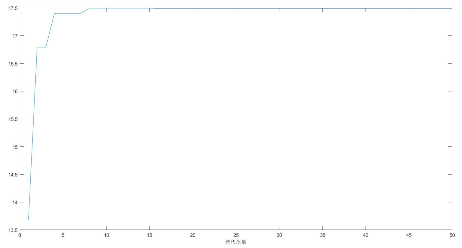
figure(2)
plot(fitnessbest) % Draw the change diagram of the best fitness for each iteration
xlabel('Number of iterations');
disp('The best location is:'); disp(gbest)
disp('At this time, the optimal value is:'); disp(Obj_fun1(gbest))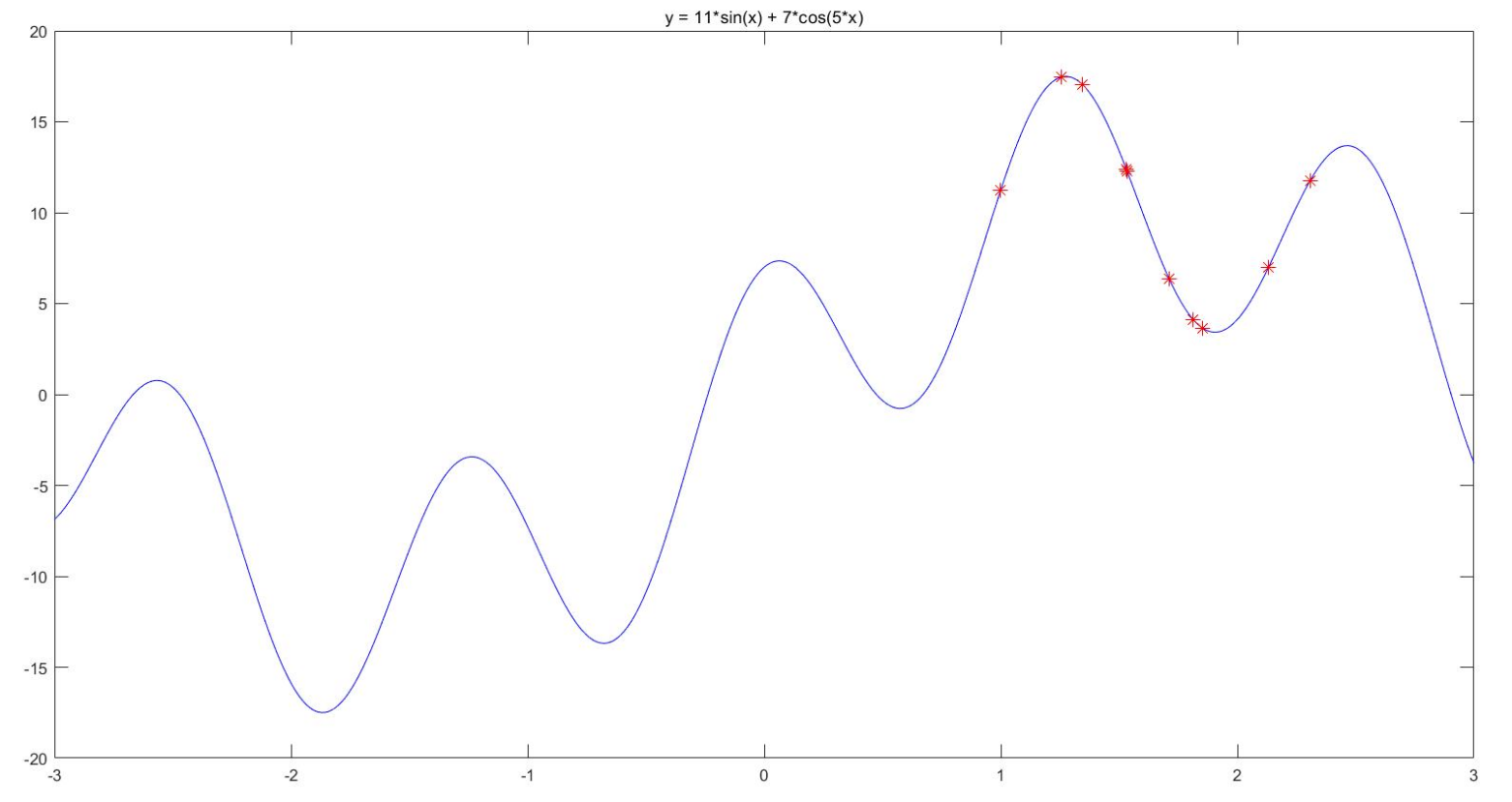
Matlab code:
%% Draw the graph of the function
x1 = -15:1:15;
x2 = -15:1:15;
[x1,x2] = meshgrid(x1,x2);
y = x1.^2 + x2.^2 - x1.*x2 - 10*x1 - 4*x2 + 60;
mesh(x1,x2,y)
xlabel('x1');  ylabel('x2');  zlabel('y');  % Label the axis
axis vis3d % Freeze the screen aspect ratio so that the rotation of a 3D object will not change the scale display of the coordinate axis
hold on

%% The parameters in the particle swarm optimization algorithm can be modified instead of the preset parameters
n = 30; % Number of particles
narvs = 2; % Number of variables
c1 = 2;  % The individual learning factor of each particle, also known as the individual acceleration constant
c2 = 2;  % The social learning factor of each particle is also called social acceleration constant
w = 0.9;  % Inertia weight
K = 100;  % Number of iterations
vmax = [6 6]; % Maximum velocity of particles
x_lb = [-15 -15]; % x Lower bound of
x_ub = [15 15]; % x Upper bound of

%% Initializes the position and velocity of particles
x = zeros(n,narvs);
for i = 1: narvs
    x(:,i) = x_lb(i) + (x_ub(i)-x_lb(i))*rand(n,1);    % The position of the randomly initialized particle is within the definition domain
end
v = -vmax + 2*vmax .* rand(n,narvs);  % The speed of randomly initialized particles (here we set it to[-vmax,vmax])

% Namely: v = -repmat(vmax, n, 1) + 2*repmat(vmax, n, 1) .* rand(n,narvs);
% be careful: x The initialization of can also be written in one line:  x = x_lb + (x_ub-x_lb).*rand(n,narvs) ,Principle and v The calculation is the same


%% Calculate fitness(Note that because it is a minimization problem, the smaller the fitness, the better)
fit = zeros(n,1);  % Initialize this n The fitness of all particles is 0
for i = 1:n  % Cycle the whole particle swarm and calculate the fitness of each particle
    fit(i) = Obj_fun2(x(i,:));   % call Obj_fun2 Function to calculate fitness
end
pbest = x;   % Initialize this n The best position a particle has found so far n*narvs (vector of)
ind = find(fit == min(fit), 1);  % Find the subscript of the particle with the least fitness
gbest = x(ind,:);  % Defines the best position all particles have found so far (a 1*narvs (vector of)

%% Mark this on the picture n The position of particles is used for demonstration
h = scatter3(x(:,1),x(:,2),fit,'*r');  % scatter3 Is a function for drawing a three-dimensional scatter chart (returned here) h In order to get the handle of the graph, we will update its position in the future)

%% iteration K To update the speed and position
fitnessbest = ones(K,1);  % Initialize the best fitness obtained in each iteration
for d = 1:K  % Start iteration, total iteration K second
    for i = 1:n   % Update page in sequence i Velocity and position of particles
        v(i,:) = w*v(i,:) + c1*rand(1)*(pbest(i,:) - x(i,:)) + c2*rand(1)*(gbest - x(i,:));  % Update page i Velocity of particles
        % If the particle's speed exceeds the maximum speed limit, adjust it
        for j = 1: narvs
            if v(i,j) < -vmax(j)
                v(i,j) = -vmax(j);
            elseif v(i,j) > vmax(j)
                v(i,j) = vmax(j);
            end
        end
        x(i,:) = x(i,:) + v(i,:); % Update page i Position of particles
        % If the particle's position exceeds the domain, adjust it
        for j = 1: narvs
            if x(i,j) < x_lb(j)
                x(i,j) = x_lb(j);
            elseif x(i,j) > x_ub(j)
                x(i,j) = x_ub(j);
            end
        end
        fit(i) = Obj_fun2(x(i,:));  % Recalculate section i Fitness of particles
        if fit(i) < Obj_fun2(pbest(i,:))   % If the first i The fitness of a particle is less than the fitness corresponding to the best position found by this particle so far
           pbest(i,:) = x(i,:);   % Then update No i The best position of particles found so far
        end
        if  fit(i) < Obj_fun2(gbest)  % If the first i The fitness of particles is less than that of all particles found so far
            gbest = pbest(i,:);   % Then update the best position all particles have found so far
        end
    end
    fitnessbest(d) = Obj_fun2(gbest);  % Update page d The best fitness obtained in this iteration
    pause(0.1)  % Pause 0.1s
    h.XData = x(:,1);  % Update the handle of the scatter chart x Axis data (at this time, the position of particles changes on the graph)
    h.YData = x(:,2);   % Update the handle of the scatter chart y Axis data (at this time, the position of particles changes on the graph)
    h.ZData = fit;  % Update the handle of the scatter chart z Axis data (at this time, the position of particles changes on the graph)
end

figure(2)
plot(fitnessbest)  % Draw the change diagram of the best fitness for each iteration
xlabel('Number of iterations');
disp('The best location is:'); disp(gbest)
disp('At this time, the optimal value is:'); disp(Obj_fun2(gbest))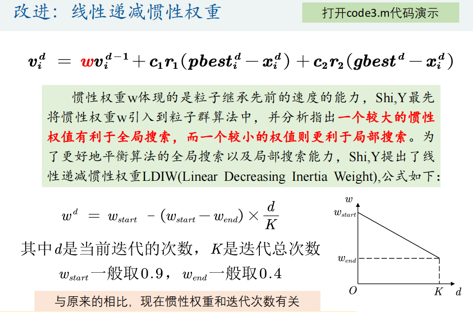

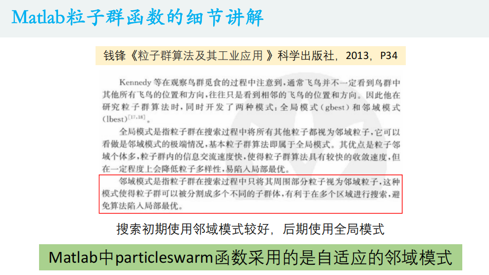
4. Particle swarm optimization function
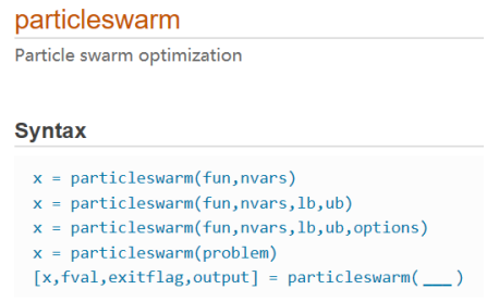
The particlewarm function is to find the minimum value. If the objective function is to find the maximum value, you need to add a negative sign to convert it to the minimum value.


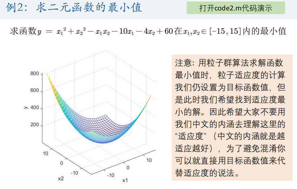
1. Solve the minimum value of function y = x1^2+x2^2-x1*x2-10*x1-4*x2+60 within [- 15,15] (the minimum value is 8)
① Write objective function
<Obj_fun2.m>
function y = Obj_fun2(x)
    y = x(1)^2 + x(2)^2 - x(1)*x(2) - 10*x(1) - 4*x(2) + 60;
end
② Solving particlewarm function
% Number of variables
narvs = 2;

% x Lower bound of(The length is equal to the number of variables, and each variable corresponds to a lower bound constraint)
x_lb = [-15 -15];

% x Upper bound of
x_ub = [15 15];

[x,fval,exitflag,output] = particleswarm(@Obj_fun2, narvs, x_lb, x_ub)
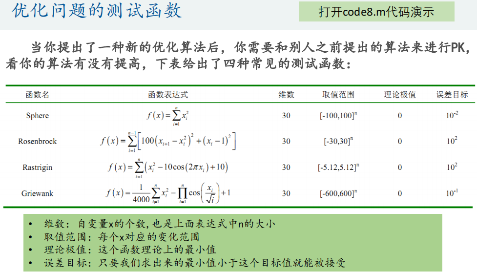
2. Call the particlewarn function to solve the test function
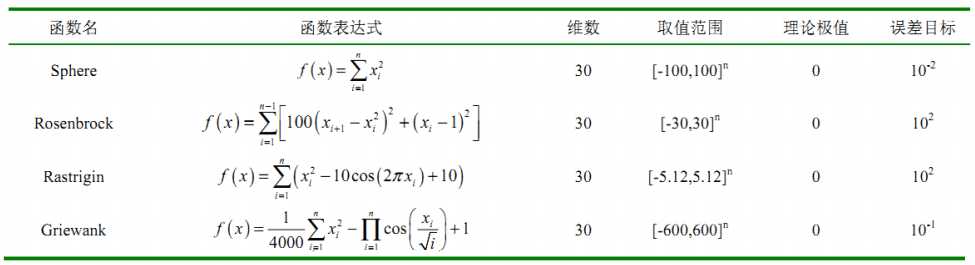
① Write objective function
<Obj_fun3.m>
function y = Obj_fun3(x)
% x Is a vector
% Sphere function
% y = sum(x.^2);
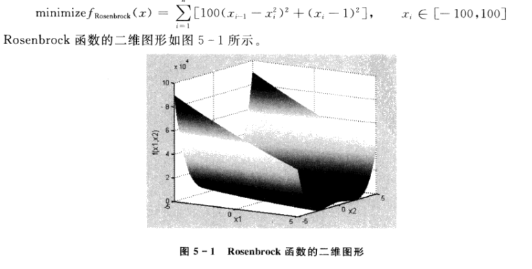
% Rosenbrock function
tem1 = x(1:end-1);
tem2 = x(2:end);
y = sum(100 * (tem2-tem1.^2).^2 + (tem1-1).^2);
% Rastrigin function
% y = sum(x.^2-10*cos(2*pi*x)+10);
% Griewank function
% y = 1/4000*sum(x.*x)-prod(cos(x./sqrt(1:30)))+1;
end
② Solving particlewarm function
narvs = 30; % Number of variables
% Sphere function
% x_lb = -100*ones(1,30); % x Lower bound of
% x_ub = 100*ones(1,30); % x Upper bound of

% Rosenbrock function
x_lb = -30*ones(1,30); % x Lower bound of
x_ub = 30*ones(1,30); % x Upper bound of

% Rastrigin function
% x_lb = -5.12*ones(1,30); % x Lower bound of
% x_ub = 5.12*ones(1,30); % x Upper bound of
% Griewank function
% x_lb = -600*ones(1,30); % x Lower bound of
% x_ub = 600*ones(1,30); % x Upper bound of

[x,fval,exitflag,output] = particleswarm(@Obj_fun3,narvs,x_lb,x_ub)
Matlab code:
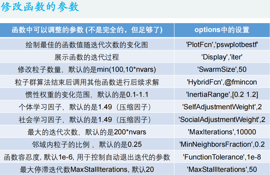
%% Draw the variation diagram of the best function value with the number of iterations
options = optimoptions('particleswarm','PlotFcn','pswplotbestf')
[x,fval] = particleswarm(@Obj_fun3,narvs,x_lb,x_ub,options)
%% Show the iterative process of the function
options = optimoptions('particleswarm','Display','iter');
[x,fval] = particleswarm(@Obj_fun3,narvs,x_lb,x_ub,options)
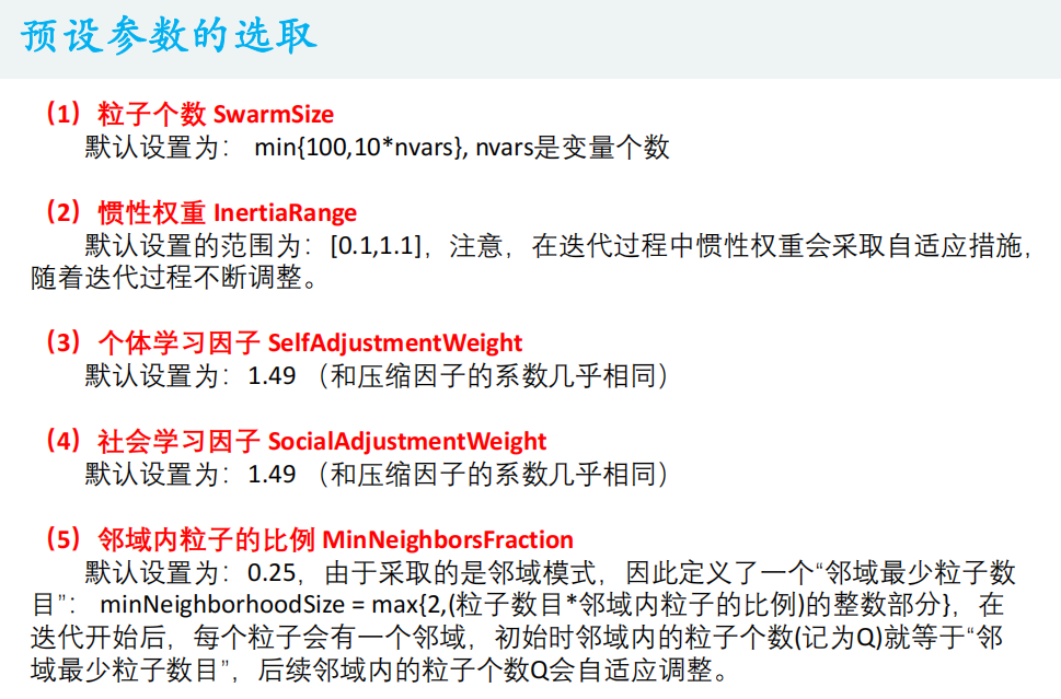
%% Modify the number of particles. The default is: min(100,10*nvars)
options = optimoptions('particleswarm','SwarmSize',50);
[x,fval] = particleswarm(@Obj_fun3,narvs,x_lb,x_ub,options)
%% After the particle swarm optimization algorithm is completed, continue to call other functions for hybrid solution( hybrid n.Mixture composition; adj.Mixed; Bastard;)
options = optimoptions('particleswarm','HybridFcn',@fmincon);
[x,fval] = particleswarm(@Obj_fun3,narvs,x_lb,x_ub,options)
%% The change range of inertia weight is 0 by default.1-1.1
options = optimoptions('particleswarm','InertiaRange',[0.2 1.2]);
[x,fval] = particleswarm(@Obj_fun3,narvs,x_lb,x_ub,options)
%% Individual learning factor, the default is 1.49(Compression factor)
options = optimoptions('particleswarm','SelfAdjustmentWeight',2);
[x,fval] = particleswarm(@Obj_fun3,narvs,x_lb,x_ub,options)
%% Social learning factor, the default is 1.49(Compression factor)
options = optimoptions('particleswarm','SocialAdjustmentWeight',2);
[x,fval] = particleswarm(@Obj_fun3,narvs,x_lb,x_ub,options)
%% The maximum number of iterations is 200 by default*nvars
options = optimoptions('particleswarm','MaxIterations',10000);
[x,fval] = particleswarm(@Obj_fun3,narvs,x_lb,x_ub,options)
%% Proportion of particles in the field MinNeighborsFraction,The default is 0.25
options = optimoptions('particleswarm','MinNeighborsFraction',0.2);
[x,fval] = particleswarm(@Obj_fun3,narvs,x_lb,x_ub,options)
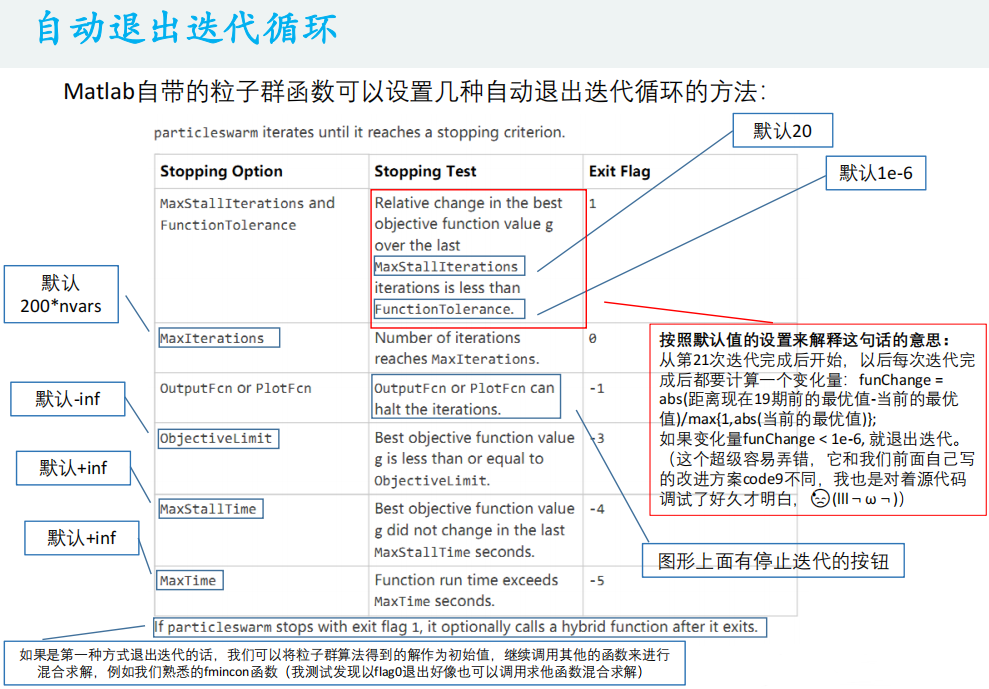
%% Function tolerance FunctionTolerance, Default 1 e-6, Parameters used to control automatic exit iteration
options = optimoptions('particleswarm','FunctionTolerance',1e-8);
[x,fval] = particleswarm(@Obj_fun3,narvs,x_lb,x_ub,options)
%% Maximum stagnant iterated algebra MaxStallIterations, Default 20, Parameters used to control automatic exit iteration
options = optimoptions('particleswarm','MaxStallIterations',50);
[x,fval] = particleswarm(@Obj_fun3,narvs,x_lb,x_ub,options)
%% The parameters controlling the exit of three iterations are modified at the same time regardless of the calculation time
tic
options = optimoptions('particleswarm','FunctionTolerance',1e-12,'MaxStallIterations',100,'MaxIterations',100000);
[x,fval] = particleswarm(@Obj_fun3,narvs,x_lb,x_ub,options)
toc
%% Other functions are called for mixed solution after the particle swarm is finished.
tic
options = optimoptions('particleswarm','FunctionTolerance',1e-12,'MaxStallIterations',50,'MaxIterations',20000,'HybridFcn',@fmincon);
[x,fval] = particleswarm(@Obj_fun3,narvs,x_lb,x_ub,options)
toc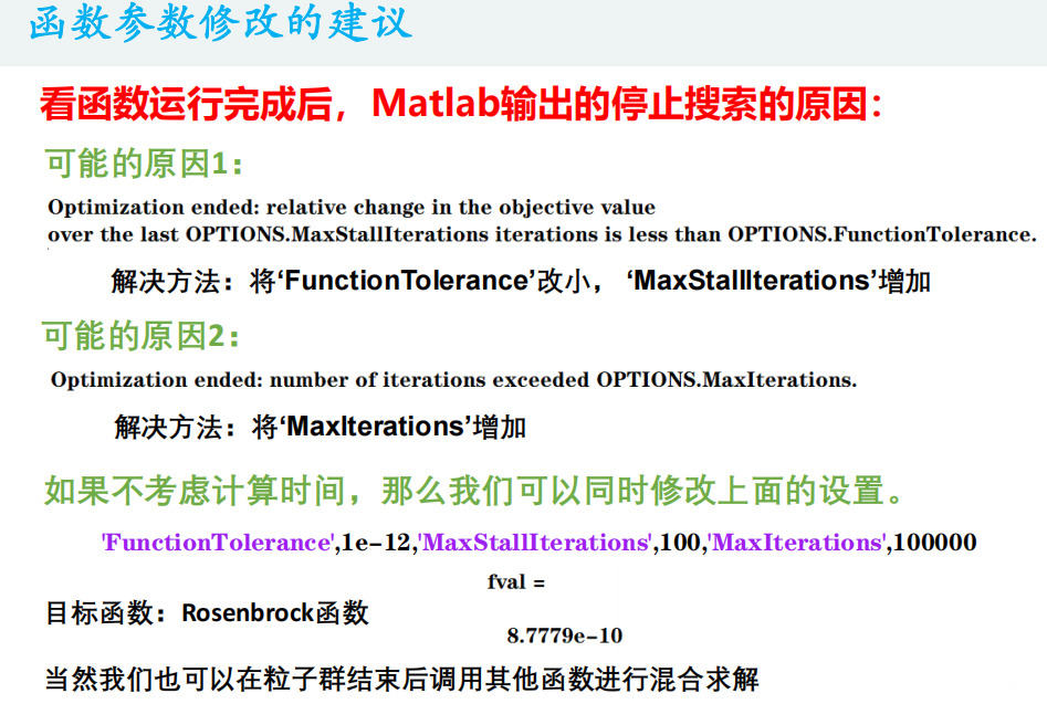

5. Advanced application of PSO algorithm
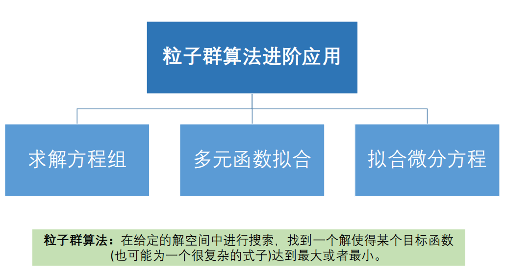
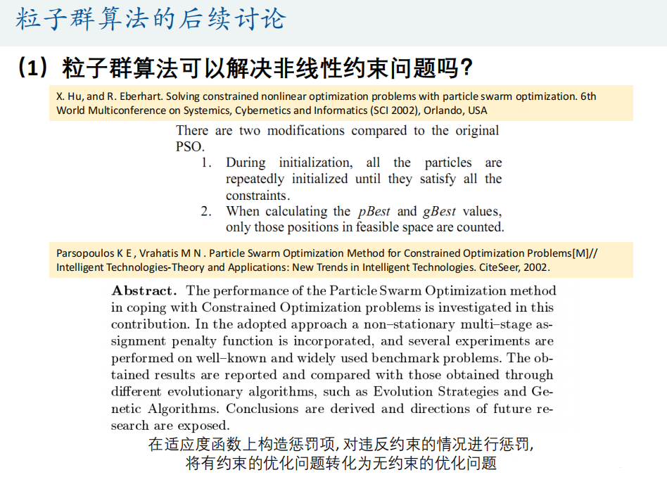
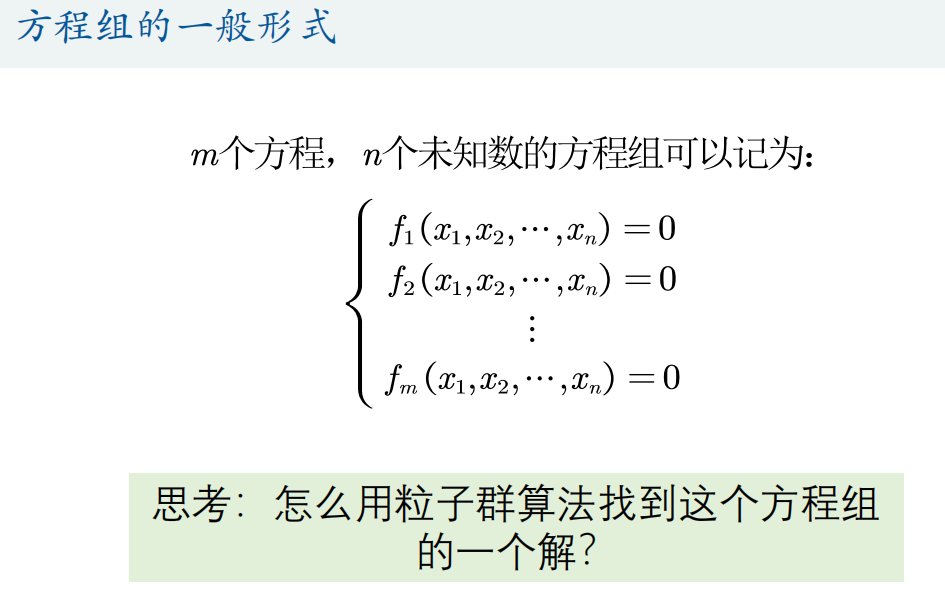
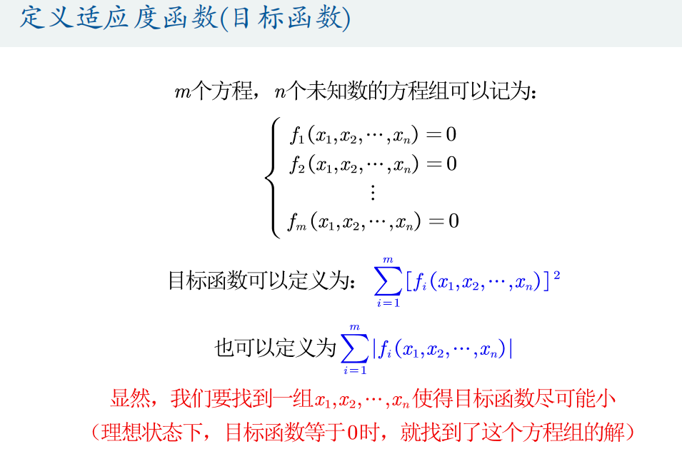
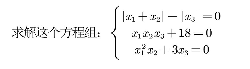
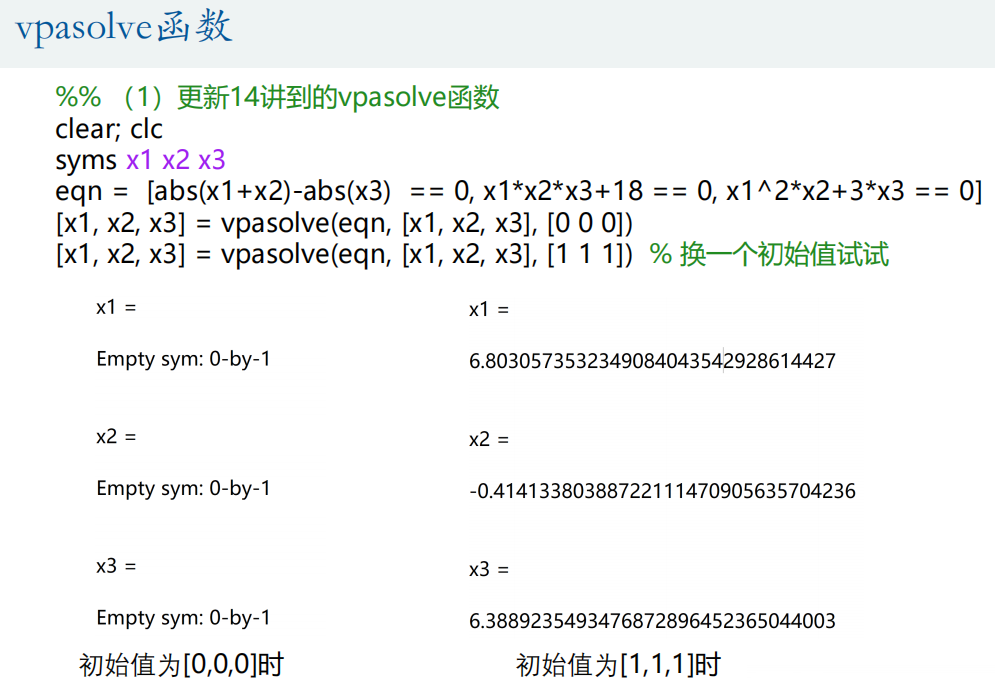
(1) Solving equations
① vpasolve function
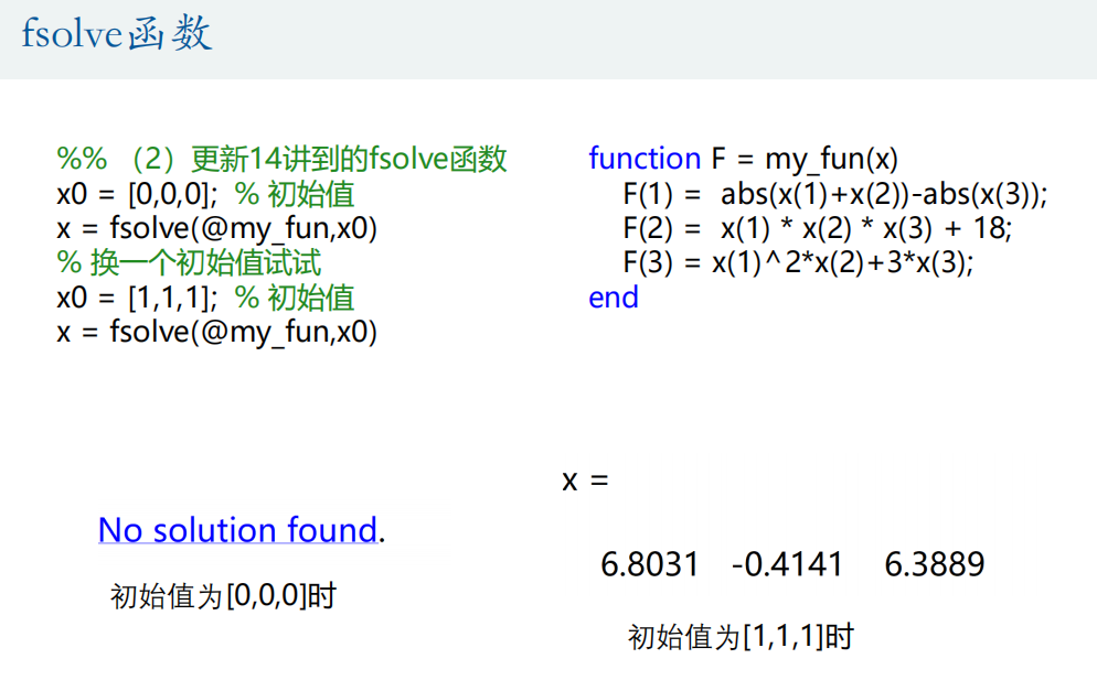
② fsolve function
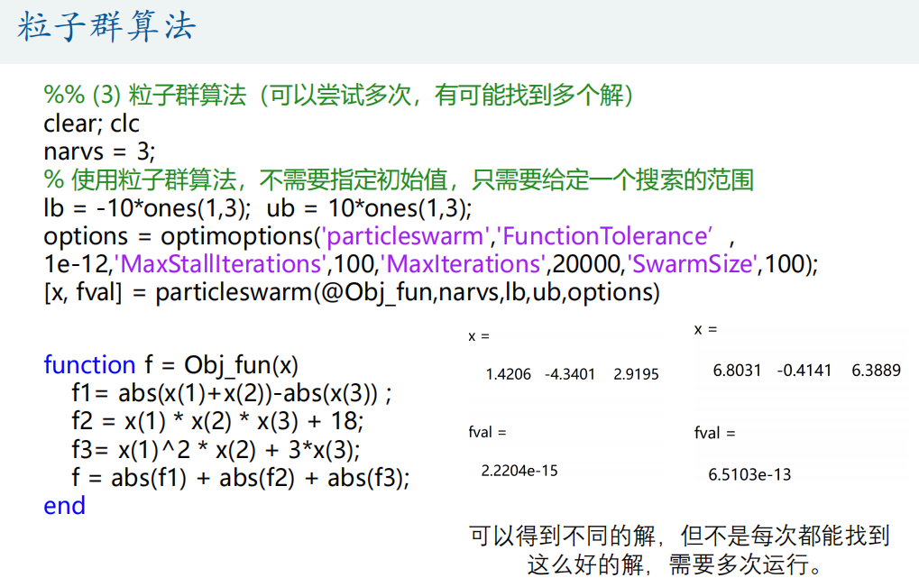
③ Particle swarm optimization

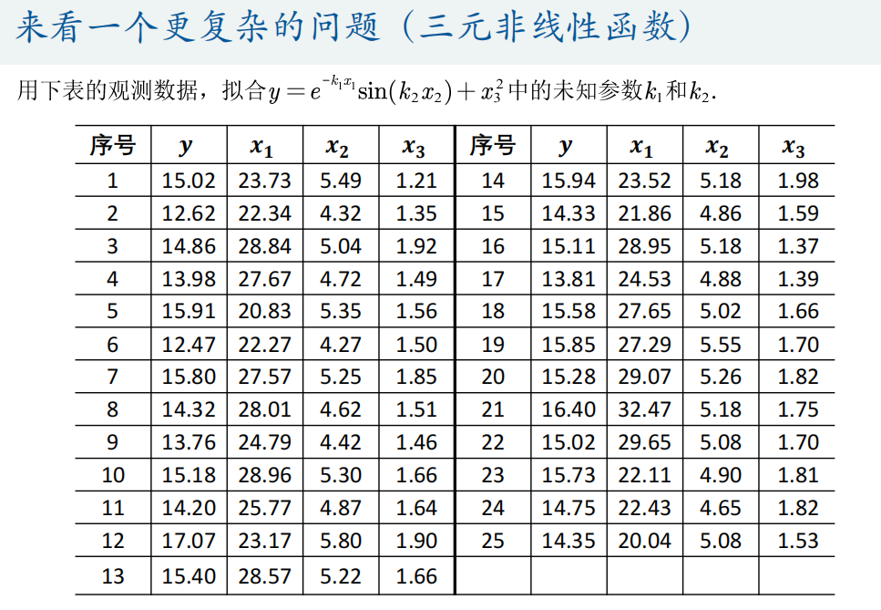
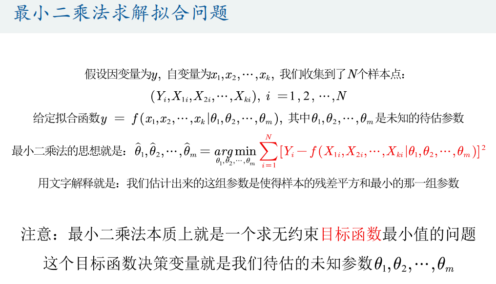
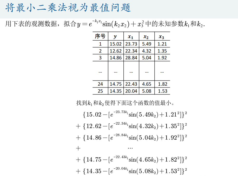
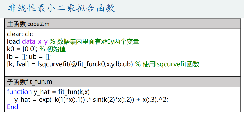
(2) Multivariate function fitting
Matlab's own fitting toolbox can only fit univariate functions and bivariate functions.
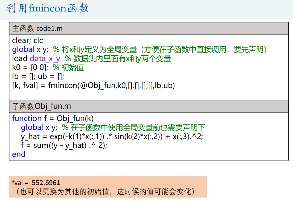
① fmincon function
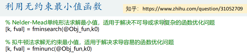
② fminsearch function and fminunc function (unconstrained)
③ lsqcurvefit function
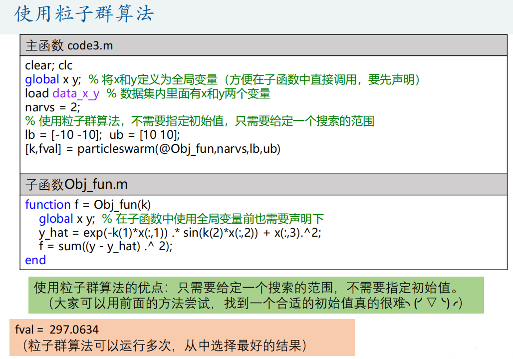
④ Particle swarm optimization
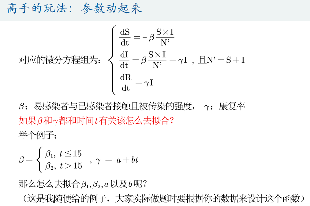
(3) Fitting differential equation
If the differential equation or system of differential equations has an analytical solution (the dsolve function can be obtained), it will be transformed into a function fitting problem, such as population prediction problem (blocking growth model);
The fitting differential equation we discussed here refers to the case that the numerical solution can only be obtained by ode45 function.
① Grid search method
<SIR_fun.m>
function dx=SIR_fun(t,x,beta,gamma)
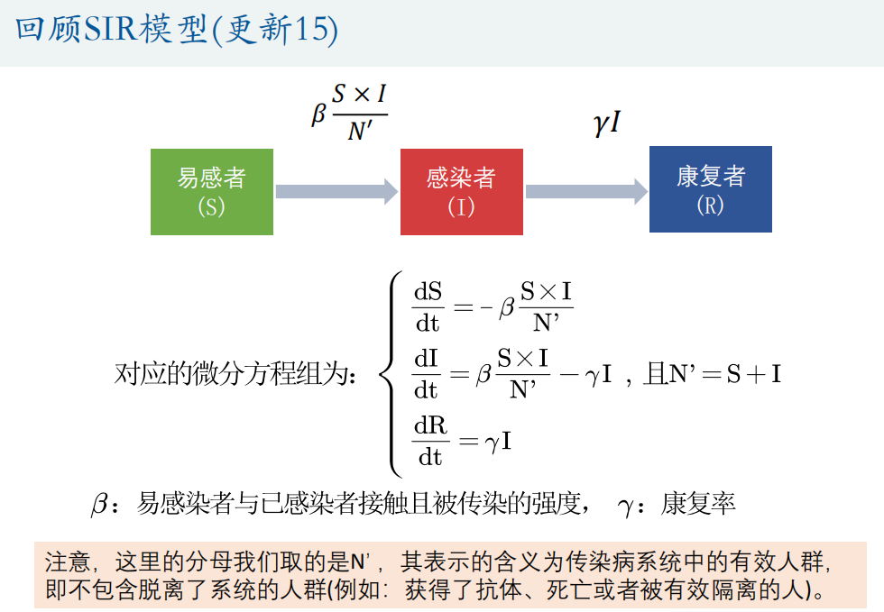
% beta: The intensity of contact between susceptible persons and infected persons
% gamma: Rehabilitation rate
dx = zeros(3,1); % x(1)express S x(2)express I x(3)express R
C = x(1)+x(2); % Effective population in infectious disease system,that is N' = S+I
dx(1) = - beta*x(1)*x(2)/C;
dx(2) = beta*x(1)*x(2)/C - gamma*x(2);
dx(3) = gamma*x(2);
end<main.m>
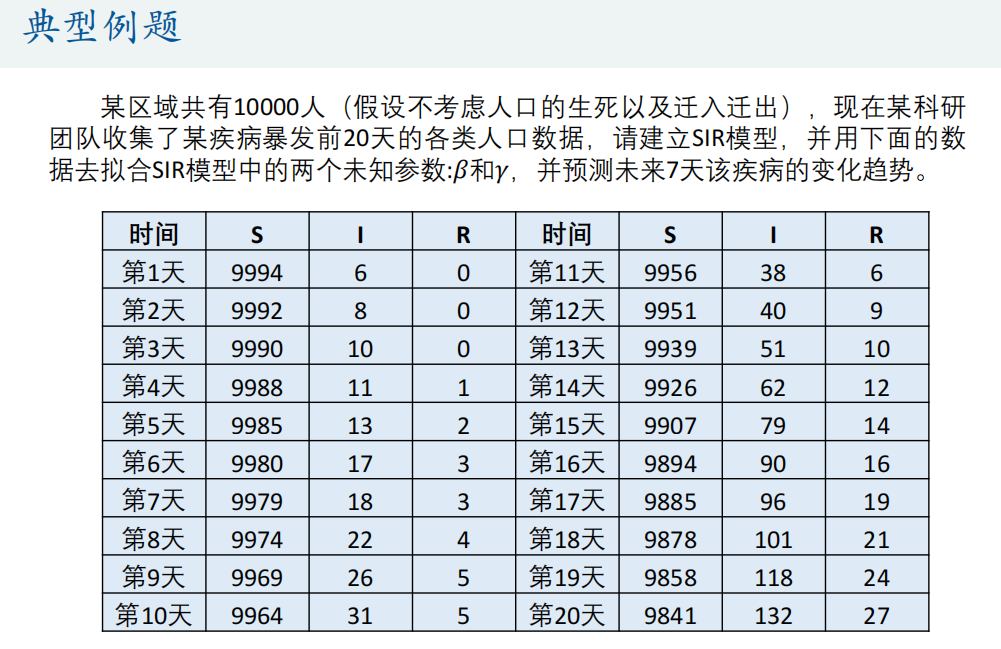
load mydata.mat % Import data (three columns in total) S,I,R (quantity of)
n = size(mydata,1); % How many rows of data are there
true_s = mydata(:,1);
true_i = mydata(:,2);
true_r = mydata(:,3);
figure(1)
plot(1:n,true_s,'r-',1:n,true_i,'b-',1:n,true_r,'g-') % S The number of is too large
legend('S','I','R')
plot(1:n,true_i,'b-',1:n,true_r,'g-') % Draw the real picture alone I and R Number of
hold on % I'll draw on this figure later
% Give a set of parameters to calculate the numerical solution of the differential equation
beta = 0.1; % The intensity of contact between susceptible persons and infected persons
gamma = 0.01; % Rehabilitation rate
[t,p]=ode45(@(t,x) SIR_fun(t,x,beta,gamma), [1:n],[true_s(1) true_i(1) true_r(1)]);
% p It is the numerical solution of the calculation. It has three columns, which are S I R Number of
p = round(p); % yes p Rounding(The number of people is an integer)
plot(1:n,p(:,2),'b--',1:n,p(:,3),'g--')
legend('I','R','Fitted I','Fitted R')
hold off
% Calculate the sum of squares of residuals
sse = sum((true_s - p(:,1)).^2 + (true_i - p(:,2)).^2 + (true_r - p(:,3)).^2)
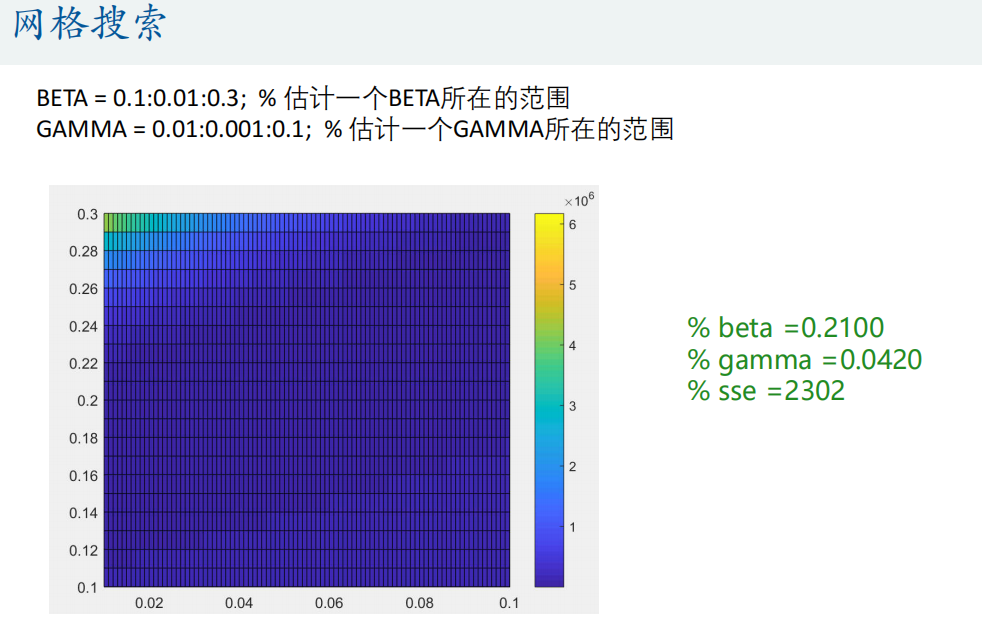
%% Grid search (enumeration method) carpet search
BETA = 0.1:0.01:0.3; % Estimate one BETA Scope
GAMMA = 0.01:0.001:0.1; % Estimate one GAMMA Scope
n1 = length(BETA);
n2 = length(GAMMA);
SSE = zeros(n1,n2); % Initialize the square sum of residuals matrix
for i = 1:n1
for j = 1:n2
beta = BETA(i);
gamma = GAMMA(j);
[t,p]=ode45(@(t,x) SIR_fun(t,x,beta,gamma), [1:n],[true_s(1) true_i(1) true_r(1)]);
% p It is the numerical solution of the calculation. It has three columns, which are S I R Number of
p = round(p); % yes p Rounding(The number of people is an integer)
% Calculate the sum of squares of residuals
sse = sum((true_s - p(:,1)).^2 + (true_i - p(:,2)).^2 + (true_r - p(:,3)).^2);
SSE(i,j) = sse;
end
end
% Draw SSE The thermodynamic diagram of this matrix appears tall in the paper
figure(2)
pcolor(GAMMA,BETA,SSE) % Attention, here GAMMA and BETA The order of cannot be reversed (similar to mesh Function usage)
colorbar % Add color bar
% find sse The smallest set of parameters
min_sse = min(min(SSE)); % min(SSE)Is to find the minimum value of each column, so we need to use it again min Function to find the minimum value in the whole matrix
[r,c] = find(SSE == min_sse,1); % find A 1 is added after it to indicate the sequence number of the row and column where the first minimum value is returned
beta = BETA(r)
gamma = GAMMA(c)
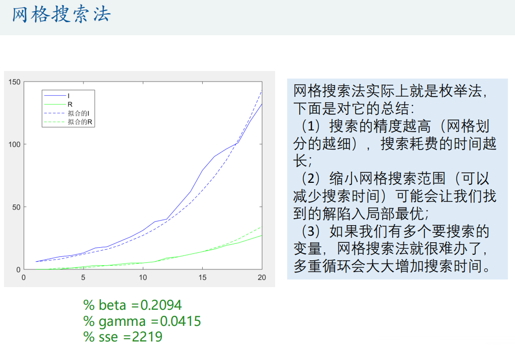
figure(3)
plot(1:n,true_i,'b-',1:n,true_r,'g-') % Draw the real picture alone I and R Number of
hold on
[t,p]=ode45(@(t,x) SIR_fun(t,x,beta,gamma), [1:n],[true_s(1) true_i(1) true_r(1)]);
% p It is the numerical solution of the calculation. It has three columns, which are S I R Number of
p = round(p); % yes p Rounding(The number of people is an integer)
plot(1:n,p(:,2),'b--',1:n,p(:,3),'g--')
legend('I','R','Fitted I','Fitted R')
hold off
% Calculate the sum of squares of residuals
sse = sum((true_s - p(:,1)).^2 + (true_i - p(:,2)).^2 + (true_r - p(:,3)).^2)
% beta =0.2100
% gamma =0.0420
% sse =2302
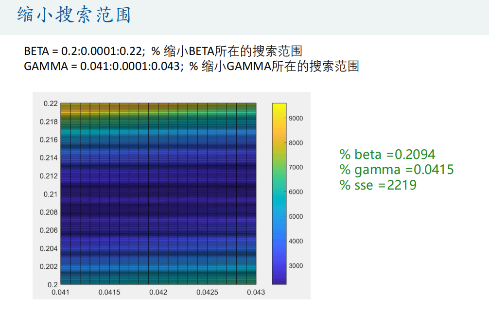
%% Think: can you make this find a better result?
BETA = 0.2:0.0001:0.22; % narrow BETA Search scope
GAMMA = 0.041:0.0001:0.043; % narrow GAMMA Search scope
% In this way, it may fall into local optimal solution
% beta =0.2094
% gamma =0.0415
% sse =2219
② Particle swarm optimization
<SIR_fun.m>
function dx=SIR_fun(t,x,beta,gamma)
     % beta: The intensity of contact between susceptible persons and infected persons
     % gamma: Rehabilitation rate
    dx = zeros(3,1);  % x(1)express S  x(2)express I  x(3)express R
    C = x(1)+x(2);  % Effective population in infectious disease system,that is N' = S+I
    dx(1) = - beta*x(1)*x(2)/C;
    dx(2) = beta*x(1)*x(2)/C - gamma*x(2);
    dx(3) = gamma*x(2);
end
<Obj_fun.m>
function f = Obj_fun(h)
    % h Is the parameter in the objective function we want to estimate
    % h The length of is the number of parameters to be estimated
    global true_s  true_i  true_r n   % Before using global variables in sub functions, you also need to declare
    beta = h(1);  % The intensity of contact between susceptible persons and infected persons
    gamma = h(2);  % Rehabilitation rate
    [t,p]=ode45(@(t,x) SIR_fun(t,x,beta,gamma), [1:n],[true_s(1) true_i(1) true_r(1)]);
    p = round(p);  % yes p Rounding(The number of people is an integer)
    % p The first column is susceptible S The number of, p The second column is the patient I The number of, p The third column of the is rehabilitation R Number of
    f = sum((true_s - p(:,1)).^2  + (true_i -  p(:,2)).^2  + (true_r - p(:,3)).^2);
end
<main.m>
load mydata.mat % Import data (three columns in total) S,I,R (quantity of)
global true_s true_i true_r n % Define global variables
n = size(mydata,1); % How many rows of data are there
true_s = mydata(:,1);
true_i = mydata(:,2);
true_r = mydata(:,3);
figure(1)
% plot(1:n,true_s,'r-',1:n,true_i,'b-',1:n,true_r,'g-') % S The number of is too large
% legend('S','I','R')
plot(1:n,true_i,'b-',1:n,true_r,'g-') % Draw separately I and R Number of
legend('I','R')
% Particle swarm optimization algorithm to solve
lb = [0 0];
ub = [1 1];
options = optimoptions('particleswarm','Display','iter','SwarmSize',100,'PlotFcn','pswplotbestf');
[h, fval] = particleswarm(@Obj_fun,2,lb,ub,options) % h The parameters to be optimized, fval Is the objective function value
% options = optimoptions('particleswarm','SwarmSize',100,'FunctionTolerance',1e-12,'MaxStallIterations',100,'MaxIterations',100000);
% [h, fval] = particleswarm(@Obj_fun,2,lb,ub,options) % h Is the parameter to be optimized, fval Is the objective function value
beta = h(1); % The intensity of contact between susceptible persons and infected persons
gamma = h(2); % Rehabilitation rate
[t,p]=ode45(@(t,x) SIR_fun(t,x,beta,gamma), [1:n],[true_s(1) true_i(1) true_r(1)]);
p = round(p); % yes p Rounding(The number of people is an integer)
sse = sum((true_s - p(:,1)).^2 + (true_i - p(:,2)).^2 + (true_r - p(:,3)).^2) % Calculate the sum of squares of residuals
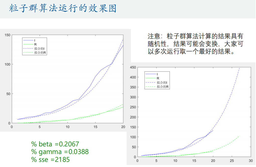
figure(3) % Put the real number and the fitted number together
plot(1:n,true_i,'b-',1:n,true_r,'g-')
hold on
plot(1:n,p(:,2),'b--',1:n,p(:,3),'g--')
legend('I','R','Fitted I','Fitted R')
% Predict future trends
N = 27; % calculation N day
[t,p]=ode45(@(t,x) SIR_fun(t,x,beta,gamma), [1:N],[true_s(1) true_i(1) true_r(1)]);
p = round(p); % yes p Rounding(The number of people is an integer)
figure(4)
plot(1:n,true_i,'b-',1:n,true_r,'g-')
hold on
plot(1:N,p(:,2),'b--',1:N,p(:,3),'g--')
legend('I','R','Fitted I','Fitted R')
③ Advanced particle swarm optimization algorithm (parameters are related to independent variables)
<SIR_fun.m>
function dx=SIR_fun(t,x,beta1,beta2,a,b)
    % beta1 : t<=15 The intensity of contact and infection between susceptible persons and infected persons
    % beta2   : t>15 The intensity of contact and infection between susceptible persons and infected persons
    % a  : Rehabilitation rate gamma = a+bt
    % b  : Rehabilitation rate gamma = a+bt
    if t <=15
        beta = beta1;
    else
        beta = beta2;
    end
    gamma = a + b * t;
    dx = zeros(3,1);  % x(1)express S  x(2)express I  x(3)express R
    C = x(1)+x(2);  % Effective population in infectious disease system,that is N' = S+I
    dx(1) = - beta*x(1)*x(2)/C;
    dx(2) = beta*x(1)*x(2)/C - gamma*x(2);
    dx(3) = gamma*x(2);
end
<Obj_fun.m>
function f = Obj_fun(h)
    % h Is the parameter in the objective function we want to estimate
    % h The length of is the number of parameters to be estimated
    global true_s  true_i  true_r n   % Before using global variables in sub functions, you also need to declare
    beta1 = h(1);  % t<=15 The intensity of contact and infection between susceptible persons and infected persons
    beta2 = h(2);  % t>15 The intensity of contact and infection between susceptible persons and infected persons
    a = h(3); % Rehabilitation rate gamma = a+bt
    b = h(4);  % Rehabilitation rate gamma = a+bt
    [t,p]=ode45(@(t,x) SIR_fun(t,x,beta1,beta2,a,b) , [1:n],[true_s(1) true_i(1) true_r(1)]);
    p = round(p);  % yes p Rounding(The number of people is an integer)
    % p The first column is susceptible S The number of, p The second column is the patient I The number of, p The third column of the is rehabilitation R Number of
    f = sum((true_s - p(:,1)).^2  + (true_i -  p(:,2)).^2  + (true_r - p(:,3)).^2);
end
<main.m>
load mydata.mat  % Import data (three columns in total) S,I,R (quantity of)
global true_s true_i true_r  n  % Define global variables
n = size(mydata,1);  % How many rows of data are there
true_s = mydata(:,1);
true_i = mydata(:,2);
true_r = mydata(:,3);
figure(1)
plot(1:n,true_i,'b-',1:n,true_r,'g-') % Draw separately I and R Number of
legend('I','R')

% Particle swarm optimization algorithm to solve
% beta1,beta2,a,b
% The search scope of given parameters (given according to the topic) can be narrowed down later
lb = [0 0 -1 -1];
ub = [1 1 1 1];
% lb = [0 0 -0.2 -0.2];
% ub = [0.3 0.3 0.2 0.2];
options = optimoptions('particleswarm','Display','iter','SwarmSize',200);
[h, fval] = particleswarm(@Obj_fun, 4, lb, ub, options)  % h The parameters to be optimized, fval Is the objective function value, The second input parameter 4 means that we have 4 variables to search

beta1 = h(1);  % t<=15 The intensity of contact and infection between susceptible persons and infected persons
beta2 = h(2);  % t>15 The intensity of contact and infection between susceptible persons and infected persons
a = h(3); % Rehabilitation rate gamma = a+bt
b = h(4);  % Rehabilitation rate gamma = a+bt
[t,p]=ode45(@(t,x) SIR_fun(t,x,beta1,beta2,a,b), [1:n],[true_s(1) true_i(1) true_r(1)]);
p = round(p);  % yes p Rounding(The number of people is an integer)

figure(3)  % Comparison drawing between the real number of people and the fitted number of people
plot(1:n,true_i,'b-',1:n,true_r,'g-')
hold on
plot(1:n,p(:,2),'b--',1:n,p(:,3),'g--')
legend('I','R','Fitted I','Fitted R')

% Predict future trends
N = 27; % calculation N day
[t,p]=ode45(@(t,x) SIR_fun(t,x,beta1,beta2,a,b), [1:N],[true_s(1) true_i(1) true_r(1)]);
p = round(p);  % yes p Rounding(The number of people is an integer)
figure(4)
plot(1:n,true_i,'b-',1:n,true_r,'g-')
hold on
plot(1:N,p(:,2),'b--',1:N,p(:,3),'g--')
legend('I','R','Fitted I','Fitted R')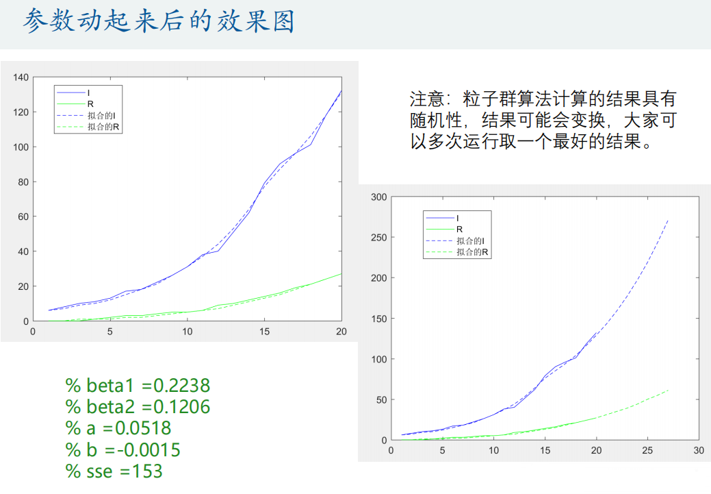
Content original author: mathematical modeling Qingfeng
Learning purpose, for reference only.