Quickly review the soft voting and hard voting in the integration method
The integration method is to combine the results of two or more separate machine learning algorithms and try to produce more accurate results than any single algorithm.
In soft voting, the probability of each category is averaged to produce results. For example, if algorithm 1 predicts that the object is a rock with 40% probability and algorithm 2 predicts that it is a rock with 80% probability, the integration will predict that the object is a rock with (80 + 40) / 2 = 60% probability.
In hard voting, the prediction of each algorithm is considered to select the set of classes with the highest number of votes. For example, if three algorithms predict the color of a particular wine as "white", "white" and "red", the integration will predict "white".
The simplest explanation is: soft voting is the integration of probability, and hard voting is the integration of result labels.
Generate test data
Let's start writing the code. First, import some libraries and some simple configurations
importpandasaspd
importnumpyasnp
importcopyascp

fromsklearn.datasetsimportmake_classification
fromsklearn.model_selectionimportKFold, cross_val_score
fromtypingimportTuple
fromstatisticsimportmode
fromsklearn.ensembleimportVotingClassifier
fromsklearn.metricsimportaccuracy_score

fromsklearn.linear_modelimportLogisticRegression
fromsklearn.ensembleimportRandomForestClassifier
fromsklearn.ensembleimportExtraTreesClassifier
fromxgboostimportXGBClassifier
fromsklearn.neural_networkimportMLPClassifier
fromsklearn.svmimportSVC
fromlightgbmimportLGBMClassifier

RANDOM_STATE : int = 42
N_SAMPLES : int = 10000
N_FEATURES : int = 25
N_CLASSES : int = 3
N_CLUSTERS_PER_CLASS : int = 2

FEATURE_NAME_PREFIX : str = "Feature"
TARGET_NAME : str = "Target"

N_SPLITS : int = 5

np.set_printoptions(suppress=True)
Some data is also needed as input for classification. make_ classification_ The dataframe function creates test data that contains features and targets.
Here we set the number of categories to 3. In this way, we can realize the soft voting and hard voting algorithms of multi classification algorithms (more than two categories can be). And our code can also be applied to binary classification.
defmake_classification_dataframe(n_samples : int = 10000, n_features : int = 25, n_classes : int = 2, n_clusters_per_class : int = 2, feature_name_prefix : str = "Feature", target_name : str = "Target", random_state : int = 42) ->pd.DataFrame:
X, y = make_classification(n_samples=n_samples, n_features=n_features, n_classes=n_classes, n_informative = n_classes*n_clusters_per_class, random_state=random_state)
feature_names = [feature_name_prefix+" "+str(v) forvinnp.arange(1, n_features+1)]
returnpd.concat([pd.DataFrame(X, columns=feature_names), pd.DataFrame(y, columns=[target_name])], axis=1)
df_data = make_classification_dataframe(n_samples=N_SAMPLES, n_features=N_FEATURES, n_classes=N_CLASSES, n_clusters_per_class=N_CLUSTERS_PER_CLASS, feature_name_prefix=FEATURE_NAME_PREFIX, target_name=TARGET_NAME, random_state=RANDOM_STATE)
X = df_data.drop([TARGET_NAME], axis=1).to_numpy()
y = df_data[TARGET_NAME].to_numpy()
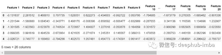
df_data.head()The data generated are as follows:
Cross validation
Use cross validation instead of train_test_split, because it can provide more robust algorithm performance evaluation.
cross_ val_ The predict helper function provides the code to do this:
defcross_val_predict(model, kfold : KFold, X : np.array, y : np.array) ->Tuple[np.array, np.array, np.array]:

    model_ = cp.deepcopy(model)

    no_classes = len(np.unique(y))

    actual_classes = np.empty([0], dtype=int)
    predicted_classes = np.empty([0], dtype=int)
    predicted_proba = np.empty([0, no_classes])

    fortrain_ndx, test_ndxinkfold.split(X):

        train_X, train_y, test_X, test_y = X[train_ndx], y[train_ndx], X[test_ndx], y[test_ndx]

        actual_classes = np.append(actual_classes, test_y)

        model_.fit(train_X, train_y)
        predicted_classes = np.append(predicted_classes, model_.predict(test_X))

        try:
            predicted_proba = np.append(predicted_proba, model_.predict_proba(test_X), axis=0)
        except:
            predicted_proba = np.append(predicted_proba, np.zeros((len(test_X), no_classes), dtype=float), axis=0)

    returnactual_classes, predicted_classes, predicted_proba
In predict_ try is added to proba because not all algorithms support probability, and there are no consistent warnings or errors that can be explicitly captured.
Before you start, take a quick look at the cross of a single algorithm_ val_ predict ..
lr = LogisticRegression(random_state=RANDOM_STATE)
kfold = KFold(n_splits=N_SPLITS, random_state=RANDOM_STATE, shuffle=True)

%timeactual, lr_predicted, lr_predicted_proba = cross_val_predict(lr, kfold, X, y)
print(f"Accuracy of Logistic Regression: {accuracy_score(actual, lr_predicted)}")
lr_predicted

Walltime: 309ms
AccuracyofLogisticRegression: 0.6821
array([0, 0, 1, ..., 0, 2, 1])
Function cross_val_predict has returned the probability and prediction category, which has been displayed in the cell output.
The first set of data is predicted to belong to 0, 0, 1, etc.
Multiple classifiers for prediction
The next thing is to generate a set of predictions and probabilities for several classifiers. The algorithms selected here are random forest, XGboost, etc
defcross_val_predict_all_classifiers(classifiers : dict) ->Tuple[np.array, np.array]:
    predictions = [None] *len(classifiers)
    predicted_probas = [None] *len(classifiers)

    fori, (name, classifier) inenumerate(classifiers.items()):
        %timeactual, predictions[i], predicted_probas[i] = cross_val_predict(classifier, kfold, X, y)
        print(f"Accuracy of {name}: {accuracy_score(actual, predictions[i])}")

    returnactual, predictions, predicted_probas

classifiers = dict()
classifiers["Random Forest"] = RandomForestClassifier(random_state=RANDOM_STATE)
classifiers["XG Boost"] = XGBClassifier(use_label_encoder=False, eval_metric='logloss', random_state=RANDOM_STATE)
classifiers["Extra Random Trees"] = ExtraTreesClassifier(random_state=RANDOM_STATE)

actual, predictions, predicted_probas = cross_val_predict_all_classifiers(classifiers)

Walltime: 17.1s
AccuracyofRandomForest: 0.8742
Walltime: 24.6s
AccuracyofXGBoost: 0.8838
Walltime: 6.2s
AccuracyofExtraRandomTrees: 0.8754
The predictions variable is a list containing a set of prediction classes for each algorithm:
[array([2, 0, 0, ..., 0, 2, 1]),
array([2, 0, 2, ..., 0, 2, 1], dtype=int64),
array([2, 0, 0, ..., 0, 2, 1])]
predict_probas is also a list, but it contains the probability of each predicted target. Each array is (10000, 3), where:
- 10000 is the number of data points in the sample data set. Each array has one row for each group of data
- 3 is the number of classes in the non binary classifier (because our goal is 3 classes)
[array([[0.17, 0.02, 0.81],
        [0.58, 0.07, 0.35],
        [0.54, 0.1 , 0.36],
        ...,
        [0.46, 0.08, 0.46],
        [0.15, 0.  , 0.85],
        [0.01, 0.97, 0.02]]),
array([[0.05611309, 0.00085733, 0.94302952],
        [0.95303732, 0.00187497, 0.04508775],
        [0.4653917 , 0.01353438, 0.52107394],
        ...,
        [0.75208634, 0.0398241 , 0.20808953],
        [0.02066649, 0.00156501, 0.97776848],
        [0.00079027, 0.99868006, 0.00052966]]),
array([[0.33, 0.02, 0.65],
        [0.54, 0.14, 0.32],
        [0.51, 0.17, 0.32],
        ...,
        [0.52, 0.06, 0.42],
        [0.1 , 0.03, 0.87],
        [0.05, 0.93, 0.02]])]
The first line in the above output is explained in detail below
For the prediction of the first set of data of the first algorithm (that is, the first row in the DataFrame has 17% probability of belonging to class 0, 2% probability of belonging to class 1 and 81% probability of belonging to class 2 (the sum of three classes is 100%).
Soft voting and hard voting
Now enter the topic of this article. Only a few lines of Python code are needed to realize soft voting and hard voting.
defsoft_voting(predicted_probas : list) ->np.array:

    sv_predicted_proba = np.mean(predicted_probas, axis=0)
    sv_predicted_proba[:,-1] = 1-np.sum(sv_predicted_proba[:,:-1], axis=1)

    returnsv_predicted_proba, sv_predicted_proba.argmax(axis=1)

defhard_voting(predictions : list) ->np.array:
    return [mode(v) forvinnp.array(predictions).T]

sv_predicted_proba, sv_predictions = soft_voting(predicted_probas)
hv_predictions = hard_voting(predictions)

fori, (name, classifier) inenumerate(classifiers.items()):
    print(f"Accuracy of {name}: {accuracy_score(actual, predictions[i])}")

print(f"Accuracy of Soft Voting: {accuracy_score(actual, sv_predictions)}")
print(f"Accuracy of Hard Voting: {accuracy_score(actual, hv_predictions)}")

AccuracyofRandomForrest: 0.8742
AccuracyofXGBoost: 0.8838
AccuracyofExtraRandomTrees: 0.8754
AccuracyofSoftVoting: 0.8868
AccuracyofHardVoting: 0.881
It can be seen from the above code that the soft voting is 0.3% higher than the single algorithm with the best performance (88.68% vs 88.38%), while the hard voting is reduced (88.10% vs 88.38%). These two mechanisms are explained in detail below
Voting algorithm code implementation
Soft voting
sv_predicted_proba = np.mean(predicted_probas, axis=0)
sv_predicted_proba

array([[0.18537103, 0.01361911, 0.80100984],
       [0.69101244, 0.07062499, 0.23836258],
       [0.50513057, 0.09451146, 0.40035798],
       ...,
       [0.57736211, 0.05994137, 0.36269651],
       [0.09022216, 0.01052167, 0.89925616],
       [0.02026342, 0.96622669, 0.01350989]])
The numpy mean function averages along the axis 0 (column). Theoretically, this should be the whole content of soft voting, because it has created the average (mean) of each of the three sets of outputs and seems to be correct.
print(np.sum(sv_predicted_proba[0]))
sv_predicted_proba[0]

0.9999999826153119
array([0.18537103, 0.01361911, 0.80100984])
However, due to the rounding error, the row values do not always add up to 1, because each data point belongs to one of the three classes with probability sum of 1
If we use the method of topk to obtain classification labels, this error will not have any impact. However, sometimes other processing is required. If the probability must be guaranteed to be 1, some simple processing needs to be done: set the value in the last column to 1 - the sum of the values in other columns
sv_predicted_proba[:,-1] = 1-np.sum(sv_predicted_proba[:,:-1], axis=1)

1.0
array([0.18537103, 0.01361911, 0.80100986])
Now there is no problem with the data. The probability of each row is 1, just as they should be.
The following is to use numpy's argmax function to obtain the category with the highest probability as the prediction result (that is, whether soft voting predicts category 0, 1 or 2 for each line).
sv_predicted_proba.argmax(axis=1)

array([2, 0, 0, ..., 0, 2, 1], dtype=int64)
The argmax function selects the index of the maximum value in the array along the axis specified in the axis parameter, so it selects 2 for the first row, 0 for the second row, 0 for the third row, etc.
Hard voting
hv_predicted = [mode(v) for v in np.array(predictions).T]
Including NP array(predictions). The T syntax simply transposes the array, changing (10000, 3) to (310000)
print(np.array(predictions).shape)
np.array(predictions).T

(3, 10000)
array([[2, 2, 2],
       [0, 0, 0],
       [0, 2, 0],
       ...,
       [0, 0, 0],
       [2, 2, 2],
       [1, 1, 1]], dtype=int64)
Then the list derivation takes each element (row) and puts statistics Mode is applied to it to select the classification that gets the most votes from the algorithm
np.array(hv_predicted)

array([2, 0, 0, ..., 0, 2, 1], dtype=int64)
Using scikit learn
Writing code from scratch can make us better the implementation mechanism of the link algorithm, but there is no need to make wheels repeatedly. Scikit learn's VotingClassifier can do all the work
estimators = list(classifiers.items())

vc_sv = VotingClassifier(estimators=estimators, voting="soft")
vc_hv = VotingClassifier(estimators=estimators, voting="hard")

%timeactual, vc_sv_predicted, vc_sv_predicted_proba = cross_val_predict(vc_sv, kfold, X, y)
%timeactual, vc_hv_predicted, _ = cross_val_predict(vc_hv, kfold, X, y)

print(f"Accuracy of SciKit-Learn Soft Voting: {accuracy_score(actual, vc_sv_predicted)}")
print(f"Accuracy of SciKit-Learn Hard Voting: {accuracy_score(actual, vc_hv_predicted)}")

Walltime: 1min4s
Walltime: 55.3s
AccuracyofSciKit-LearnSoftVoting: 0.8868
AccuracyofSciKit-LearnHardVoting: 0.881
The results of cikit learn implementation are exactly the same as our handwritten algorithm - the accuracy of soft voting is 88.68%, and the accuracy of hard voting is 88.1%.
Why is hard voting ineffective?
Consider this situation. Take binary classification as an example:
The probabilities of B are 0.01, 0.51, 0.6, 0.1 and 0.7 respectively, then
The probability of A is 0.99, 0.49, 0.4, 0.9, 0.3
If calculated by hard voting:
B 3 votes, a 2 votes, the result is B
Calculation of soft voting
B: (0.01+0.51+0.6+0.1+0.7)/5=0.38
A:(0.99+0.49+0.4+0.9+0.3)/5=0.61
The result is A
The result of hard voting is ultimately determined by the model with relatively low probability value (0.51, 0.6, 0.7), while soft voting is determined by the model with higher probability value (0.99, 0.9). Soft voting will give those models with high probability more weight, so it performs better than hard voting.
How much can integrated learning improve?
Let's see how much improvement ensemble learning can achieve in accuracy measurement? See how many of the six common extrusion algorithms we can use
lassifiers = dict()
classifiers["Random Forrest"] = RandomForestClassifier(random_state=RANDOM_STATE)
classifiers["XG Boost"] = XGBClassifier(use_label_encoder=False, eval_metric='logloss', random_state=RANDOM_STATE)
classifiers["Extra Random Trees"] = ExtraTreesClassifier(random_state=RANDOM_STATE)
classifiers['Neural Network'] = MLPClassifier(max_iter = 1000, random_state=RANDOM_STATE)
classifiers['Support Vector Machine'] = SVC(probability=True, random_state=RANDOM_STATE)
classifiers['Light GMB'] = LGBMClassifier(random_state=RANDOM_STATE)

estimators = list(classifiers.items())
Method 1: use handwritten code
%time
actual, predictions, predicted_probas = cross_val_predict_all_classifiers(classifiers) # Get a collection of predictions and probabilities from the selected algorithms

sv_predicted_proba, sv_predictions = soft_voting(predicted_probas) # Combine those collections into a single set of predictions
hv_predictions = hard_voting(predictions)

print(f"Accuracy of Soft Voting: {accuracy_score(actual, sv_predictions)}")
print(f"Accuracy of Hard Voting: {accuracy_score(actual, hv_predictions)}")

Walltime: 14.9s
AccuracyofRandomForest: 0.8742
Walltime: 32.8s
AccuracyofXGBoost: 0.8838
Walltime: 5.78s
AccuracyofExtraRandomTrees: 0.8754
Walltime: 3min2s
AccuracyofNeuralNetwork: 0.8612
Walltime: 36.2s
AccuracyofSupportVectorMachine: 0.8674
Walltime: 1.65s
AccuracyofLightGMB: 0.8828
AccuracyofSoftVoting: 0.8914
AccuracyofHardVoting: 0.8851
Walltime: 4min34s
Method 2: use scikit learn and cross_val_predict
%%time
vc_sv = VotingClassifier(estimators=estimators, voting="soft")
vc_hv = VotingClassifier(estimators=estimators, voting="hard")

%timeactual, vc_sv_predicted, vc_sv_predicted_proba = cross_val_predict(vc_sv, kfold, X, y)
%timeactual, vc_hv_predicted, _ = cross_val_predict(vc_hv, kfold, X, y)

print(f"Accuracy of SciKit-Learn Soft Voting: {accuracy_score(actual, vc_sv_predicted)}")
print(f"Accuracy of SciKit-Learn Hard Voting: {accuracy_score(actual, vc_hv_predicted)}")

Walltime: 4min11s
Walltime: 4min41s
AccuracyofSciKit-LearnSoftVoting: 0.8914
AccuracyofSciKit-LearnHardVoting: 0.8859
Walltime: 8min52s
Method 3: use scikit learn and cross_val_score
%timeprint(f"Accuracy of SciKit-Learn Soft Voting using cross_val_score: {np.mean(cross_val_score(vc_sv, X, y, cv=kfold))}")

AccuracyofSciKit-LearnSoftVotingusingcross_val_score: 0.8914
Walltime: 4min46s
Three different methods have reached an agreement on the accuracy of soft voting, which once again shows that our handwritten implementation is correct.
Supplement: restrictions on scikit learn hard voting
fromcatboostimportCatBoostClassifier
fromsklearn.model_selectionimportcross_val_score

classifiers["Cat Boost"] = CatBoostClassifier(silent=True, random_state=RANDOM_STATE)
estimators = list(classifiers.items())

vc_hv = VotingClassifier(estimators=estimators, voting="hard")

print(cross_val_score(vc_hv, X, y, cv=kfold))
You will get an error:
ValueError: couldnotbroadcastinputarrayfromshape (2000,1) intoshape (2000)
This problem is easy to solve because the output is (2000, 1) and the input requirement is (2000), so we can use NP Squeeze delete the second dimension.
summary
By adding neural network, support vector machine and lightGMB into the combination, the accuracy of soft voting is improved by 0.46% to 89.14% from 88.68%, and the accuracy of the new soft voting is 0.76% higher than that of the best individual algorithm (XG Boost is 88.38). Adding Light GMB whose accuracy score is lower than XGBoost improves the integration performance by 0.1%! In other words, integration is not the best model, which can also improve the performance of soft voting. If it's a Kaggle game, then 0.76% may be huge, which may make you leap on the leaderboard.
https://www.overfit.cn/post/a4a0f83dafad46f3b4135b5faf1ca85a
By Graham Harrison