16_NLP stateful CharRNN_window_Tokenizer_stationary_colab_ResetState_character word level_regex_IMDb: https://blog.csdn.net/Linli522362242/article/details/115388298
16_2NLP RNN_colab tensorboard_os.curdir_Pretrained Embed_TrainingSampler_En–Decoder_Beam search_mask: https://blog.csdn.net/Linli522362242/article/details/115518150
16_3_NLP RNNs Encoder Decoder Multi-Head Attention_complexity_max path length_sequential operations_colorbar:https://blog.csdn.net/Linli522362242/article/details/115689038
Exercises
1. What are the pros and cons of using a stateful RNN versus a stateless RNN?
- Stateless RNNs(at each training iteration the model starts with a hidden state full of zeros, then it updates this state at each time step, and after the last time step, it throws it away, as it is not needed anymore.) can only capture patterns whose length is less than, or equal to, the size of the windows the RNN is trained on. Conversely,
- stateful RNNs can capture longer-term patterns. However, implementing a stateful RNN is much harder—especially preparing the dataset properly. Moreover, stateful RNNs do not always work better, in part because consecutive batches are not independent and identically distributed (IID). Gradient Descent is not fond of non-IID datasets.
2. Why do people use Encoder–Decoder RNNs rather than plain sequence-to-sequence RNNs for automatic translation?
In general, if you translate a sentence one word at a time, the result will be terrible. For example, the French sentence "Je vous en prie" means "You are welcome," but if you translate it one word at a time, you get "I you in pray." Huh? It is much better to read the whole sentence first and then translate it. A plain sequence-tosequence RNN would start translating a sentence immediately after reading the first word, while an Encoder–Decoder RNN will first read the whole sentence and then translate it. That said, one could imagine a plain sequence-to-sequence RNN that would output silence whenever it is unsure about what to say next (just like human translators do when they must translate a live broadcast).
3. How can you deal with variable-length input sequences? What about variable length output sequences?
Variable-length input sequences can be handled by padding the shorter sequences so that all sequences in a batch have the same length, and using masking to ensure the RNN ignores the padding token. For better performance, you may also want to create batches containing sequences of similar sizes. Ragged tensors can hold sequences of variable lengths, and tf.keras will likely support them eventually, which will greatly simplify handling variable-length input sequences (at the time of this writing, it is not the case yet).
Regarding variable-length output sequences,
- if the length of the output sequence is known in advance (e.g., if you know that it is the same as the input sequence), then you just need to configure the loss function so that it ignores tokens that come after the end of the sequence. Similarly, the code that will use the model should ignore tokens beyond the end of the sequence.
- But generally the length of the output sequence is not known ahead of time, so the solution is to train the model so that it outputs an end of sequence token at the end of each sequence.
4. What is beam search and why would you use it? What tool can you use to implement it?
Beam search is a technique used to improve the performance of a trained Encoder–Decoder model, for example in a neural machine translation system. The algorithm
- keeps track of a short list of the k most promising output sentences (say, the top three), and at each decoder step it tries to extend them by one word(token);
- then it keeps only the k most likely sentences.https://blog.csdn.net/Linli522362242/article/details/115518150
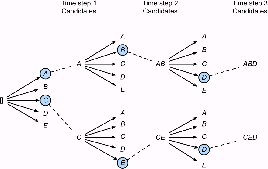 Beam search is an improved version of greedy search. It has a hyperparameter named beam size, k. At time step 1, we select k tokens with the highest conditional probabilities. Each of them will be the first token of k candidate output sequences, respectively. At each subsequent time step, based on the k candidate output sequences at the previous time step, we continue to select k candidate output sequences with the highest conditional probabilities from
  possible choices.
 - The parameter k is called the beam width: the larger it is, the more CPU and RAM will be used, but also the more accurate the system will be. Instead of greedily choosing the most likely next word at each step to extend a single sentence, this technique allows the system to explore several promising sentences simultaneously. Moreover, this technique lends itself well to parallelization. You can implement beam search fairly easily using TensorFlow Addons.
5. What is an attention mechanism? How does it help?
 https://blog.csdn.net/Linli522362242/article/details/115689038
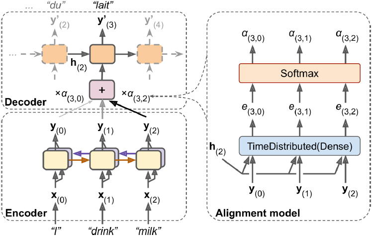
An attention mechanism is a technique initially used in Encoder–Decoder models to give the decoder more direct access to the input sequence, allowing it to
deal with longer input sequences. At each decoder time step, the current decoder's state and the full output of the encoder are processed by an alignment model that outputs an alignment score(e.g. ) for each input time step(t). This score indicates which part of the input is most relevant to the current decoder time step.
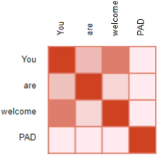 https://blog.csdn.net/Linli522362242/article/details/115689038
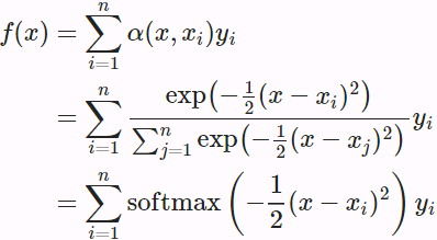
The weighted sum of the encoder output  (weighted by their alignment score
 or
or  ) is then fed to the decoder, which produces the next decoder state and the output for this time step.
- The main benefit of using an attention mechanism is the fact that the Encoder–Decoder model can successfully process longer input sequences.
- Another benefit is that the alignment scores makes the model easier to debug and interpret(This is called explainability): for example, if the model makes a mistake, you can look at which part of the input it was paying attention to, and this can help diagnose the issue.(for example, if an image of a dog walking in the snow is labeled as "a wolf walking in the snow," then you can go back and check what the model focused on when it output the word "wolf." You may find that it was paying attention not only to the dog, but also to the snow, hinting at a possible explanation: perhaps the way the model learned to distinguish dogs from wolves is by checking whether or not there's a lot of snow around. You can then fix this by training the model with more images of wolves without snow, and dogs with snow.) An attention mechanism is also at the core of the Transformer architecture, in the Multi-Head Attention layers. See the next answer.
6. What is the most important layer in the Transformer architecture? What is its purpose?
The most important layer in the Transformer architecture is the Multi-Head Attention layer (the original Transformer architecture contains18 of them,
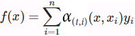
including 6 Masked Multi-Head Attention layers).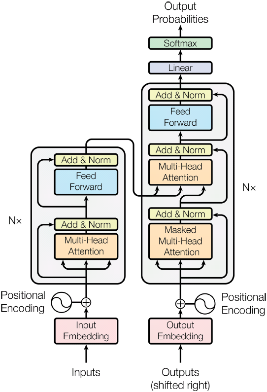
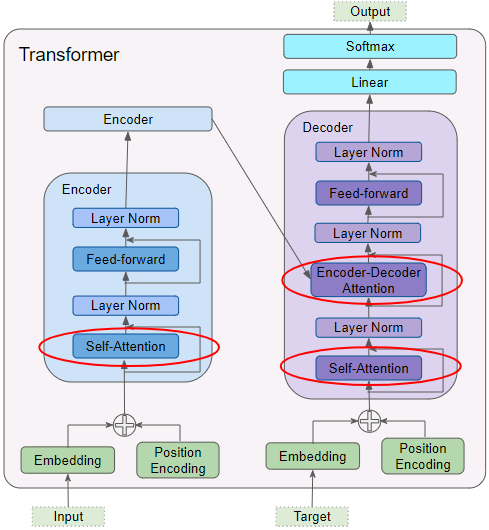
It is at the core of language models such as BERT and GPT-2. Its purpose is to allow the model to identify which words are most aligned with each other, and then improve each word's representation using these contextual clues.
7. When would you need to use sampled softmax?
Sampled softmax is used when training a classification model when there are many classes (e.g., thousands)(When the output vocabulary is large (which is the case here), outputting a probability for each and every possible word would be terribly slow. If the target vocabulary contains, say, 50,000 French words, then the decoder would output 50,000-dimensional vectors, and then computing the softmax function over such a large vector would be very computationally intensive. To avoid this,https://blog.csdn.net/Linli522362242/article/details/115518150). It computes an approximation of the crossentropy loss based on the logit predicted by the model for the correct word, and the predicted logits for a sample of incorrect words. This speeds up training considerably compared to computing the softmax over all logits and then estimating the cross-entropy loss. After training, the model can be used normally, using the regular softmax function to compute all the class probabilities based on all the logits.
In TensorFlow you can use the tf.nn.sampled_softmax_loss() function for this during training and use the normal softmax function at inference time (sampled softmax cannot be used at inference time because it requires knowing the target).
8. Embedded Reber grammars were used by Hochreiter and Schmidhuber in their paper about LSTMs https://scholar.google.com/scholar?q=Long+Short-Term+Memory+author%3ASchmidhuber. They are artificial grammars that produce strings such as "BPBTSXXVPSEPE." Check out Jenny Orr's nice introduction to this topic https://www.willamette.edu/~gorr/classes/cs449/reber.html. Choose a particular embedded Reber grammar (such as the one represented on Jenny Orr's page), then train an RNN to identify whether a string respects that grammar or not. You will first need to write a function capable of generating a training batch containing about 50% strings that respect the grammar, and 50% that don't.
First we need to build a function that generates strings based on a Reber grammar. The grammar will be represented as a list of possible transitions for each state. A transition specifies the string to output (or a grammar to generate it) and the next state. We start at B, and move from one node(state_i) to the next, adding the symbols we pass to our string as we go. When we reach the final E, we stop. If there are two paths we can take, e.g. after T we can go to either S or X, we randomly choose one (with equal probability).
default_reber_grammar = [
    [("B", 1)],          #(state 0) output=B ==>(state 1)
    [("T", 2), ("P", 3)],#(state 1) output=T ==>(state 2) OR =P ==>(state 3)
    [("S", 2), ("X", 4)],#(state 2) output=S ==>(state 2) OR =X ==>(state 4)
    [("T", 3), ("V", 5)],# and so on...
    [("X", 3), ("S", 6)],
    [("P", 4), ("V", 6)],
    [("E", None)]]        #(state 6) output=E ==>(terminal state)
In this manner we can generate an infinite number of strings which belong to the rather peculiar Reber language. Verify for yourself that the strings on the left below are possible Reber strings, while those on the right are not.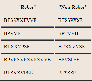 What are the set of symbols which can "legally" follow a T?. An S can follow a T, but only if the immediately preceding symbol was a B.
 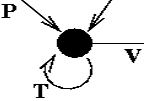 A V or a T can follow a T, but only if the symbol immediately preceding it was either a T or a P(e.g. PTT, PTV, PTTV, PTTT, ...). In order to know what symbol sequences are legal, therefore, any system which recognizes reber strings must have some form of memory, which can use not only the current input, but also fairly recent history in making a decision.
Let's generate a few strings based on the default Reber grammar:
np.random.seed(42)

def generate_string( grammar ):
    state = 0 # state: node
    output = []
    while state is not None:  # or the number of choice output after state
        index = np.random.randint( len(grammar[state]) )
        production, state = grammar[state][index]
#         if isinstance(production, list):# for embedded_reber_grammar
#             production = generate_string( grammar=production)
        output.append(production)
    return "".join(output)

for _ in range(25):
    print(generate_string(default_reber_grammar), end=" ")
Looks good.
While the Reber grammar represents a simple finite state grammar and has served as a benchmark for equally simple learning systems (it can be learned by an Elman network), a more demanding task is to learn the Embedded Reber Grammar, shown below: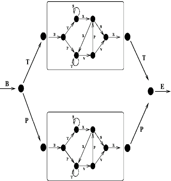 Using this grammar two types of strings are generated: one kind which is made using the top path through the graph: BT<reber string>TE and one kind made using the lower path: BP<reber string>PE. To recognize these as legal strings, and learn to tell them from illegal strings such as BP<reber string>TE, a system must be able to remember the second symbol of the series, regardless of the length of the intervening input (which can be as much as 50 or more symbols), and to compare it with the second last symbol seen. An Elman network can no longer solve this task, but RTRL (Real Time Recurrent Learning) can usually solve it (with some difficulty). We will discuss both of these next. More recent recurrent models can always solve it.
embedded_reber_grammar = [
    [("B", 1)],
    [("T", 2), ("P", 3)],
    [(default_reber_grammar, 4)],
    [(default_reber_grammar, 5)],
    [("T", 6)],
    [("P", 6)],
    [("E", None)]]

import numpy as np

def generate_string( grammar ):
    state = 0 # state: node
    output = []
    while state is not None:  # or the number of choice output after state
        index = np.random.randint( len(grammar[state]) )
        production, state = grammar[state][index]
        if isinstance(production, list):# for embedded_reber_grammar
            production = generate_string( grammar=production)
        output.append(production)
    return "".join(output)
Now let's generate a few strings based on the embedded Reber grammar:
np.random.seed(42)
for _ in range(25):
print(generate_string(embedded_reber_grammar), end=" ")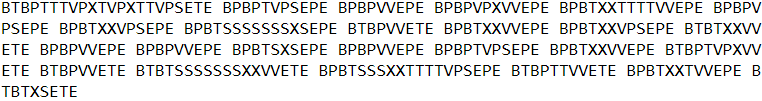 Okay,
Okay,
now we need a function to generate strings that do not respect the grammar. We could generate a random string, but the task would be a bit too easy, so instead we will generate a string that respects the grammar, and we will corrupt it by changing just one character:
POSSIBLE_CHARS = "BEPSTVX"

def generate_corrupted_string( grammar, chars=POSSIBLE_CHARS ):
    good_string = generate_string( grammar )
    index = np.random.randint( len(good_string) )
    good_char = good_string[index]
    # changing just one character
    bad_char = np.random.choice( sorted(set(chars)-set(good_char)) )
    return good_string[:index] + bad_char + good_string[index+1:]

# Let's look at a few corrupted strings:
np.random.seed(42)

for _ in range(25):
    print( generate_corrupted_string(embedded_reber_grammar),
           end=" " )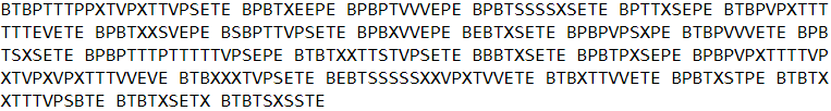
We cannot feed strings directly to an RNN, so we need to encode them somehow.
- One option would be to one-hot encode each character.
- Another option is to use embeddings.
- Let's go for the second option (but since there are just a handful of characters, one-hot encoding would probably be a good option as well). For embeddings to work, we need to convert each string into a sequence of character IDs. Let's write a function for that, using each character's index in the string of possible characters "BEPSTVX":
def string_to_ids(s, chars=POSSIBLE_CHARS):
    return [chars.index(c) for c in s]

string_to_ids("BTTTXXVVETE") 
We can now generate the dataset, with 50% good strings, and 50% bad strings:
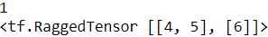
###########################
# RaggedTensor
https://www.tensorflow.org/guide/ragged_tensor?hl=zh-cn
broadcasting
# x       (2D ragged):  2 x (num_rows)
# y       (scalar)
# result  (2D ragged):  2 x (num_rows)
x = tf.ragged.constant([[1, 2], [3]]) # 2xr1
y = 3
print(x.ragged_rank) #==>1
print(x + y)
 # the irregular rank of the # irregular tensor is the number of partitions of the underlying # values # tensor (i.e. the nesting depth of the # RaggedTensor # object)
#The number of partitions of the x ^ values ^ tensor is ragged_rank=1
# x         (2d ragged):  3 x (num_rows)
# y         (2d tensor):  3 x          1
# Result    (2d ragged):  3 x (num_rows)
x = tf.ragged.constant([
                        [10, 87, 12],
                        [19, 53],
                        [12, 32]
                       ])# 3x r1
y = [[1000], [2000], [3000]]
print(x.ragged_rank) # ==> 1
print(x + y)
==>Because y is 3x1, press 3x # r1 to broadcast
#The number of partitions of the x ^ values ^ tensor is ragged_rank=1
# trailing dimensions do not match.##########
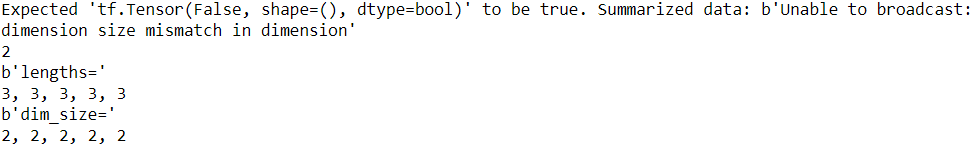
# x      (2d ragged): 3 x (r1)
# y      (2d tensor): 3 x   4  # trailing dimensions do not match.##########
x = tf.ragged.constant([[1, 2], [3, 4, 5, 6], [7]]) # 2,4,1
y = tf.constant([[1, 2, 3, 4], [5, 6, 7, 8], [9, 10, 11, 12]]) # 4,4,4
try:
  x + y
except tf.errors.InvalidArgumentError as exception:
  print(exception)
Expected 'tf.Tensor(False, shape=(), dtype=bool)' to be true. Summarized data: b'Unable to broadcast: dimension size mismatch in dimension'
1
b'lengths='
4
b'dim_size='
2, 4, 1
#The ragged_rank of the irregular tensor is the number of partitions of the underlying # values # tensor (i.e. the nesting depth of the # RaggedTensor # object)
#The number of partitions of the x ^ values ^ tensor is ragged_rank=1
# ragged dimensions do not match.##########
# x      (2d ragged): 3 x (r1)
# y      (2d ragged): 3 x (r2)  # ragged dimensions do not match.##########
x = tf.ragged.constant([[1, 2, 3], [4], [5, 6]]) # 3, 1, 2
y = tf.ragged.constant([[10, 20], [30, 40], [50]]) # 2, 2, 1
try:
  x + y
except tf.errors.InvalidArgumentError as exception:
  print(exception)
Expected 'tf.Tensor(False, shape=(), dtype=bool)' to be true. Summarized data: b'Unable to broadcast: dimension size mismatch in dimension'
1
b'lengths='
2, 2, 1
b'dim_size='
3, 1, 2
#The number of partitions of the x,y values tensor is ragged_rank=1
# x      (3d ragged): 3 x (r1) x 2
# y      (3d ragged): 3 x (r1) x 3  # trailing dimensions do not match ##########
x = tf.ragged.constant([[[1, 2], [3, 4], [5, 6]],
                        [[7, 8], [9, 10]]]) # 2, 2, 2, 2, 2
y = tf.ragged.constant([[[1, 2, 0], [3, 4, 0], [5, 6, 0]],
                        [[7, 8, 0], [9, 10, 0]]]) # 3, 3, 3, 3, 3
print(x.ragged_rank) #==> 2
print(y.ragged_rank) #==> 2
try:
  x + y
except tf.errors.InvalidArgumentError as exception:
  print(exception)
# x,y # the number of partitions of the # values # tensor is ragged_rank=2?
# x,y # the number of partitions of the underlying # values # tensor (pylist: A nested # list, tuple # or # np.ndarray. Their underlying nested element # is a scalar value) is ragged_rank=2?
rt = tf.RaggedTensor.from_row_splits(
    values=tf.RaggedTensor.from_row_splits(
       #index= 0 1 2 3 4 5 6 7 8 9  10
        values=[1,2,3,4,5,6,7,8,9,10],  #index:0     1      2     3      4       5
        row_splits=[0, 2, 4, 6, 8, 10]), # ==> [0,2), [2,4), [4,6), [6,8), [8,10)
    row_splits=[0, 3,  5])
print(rt)
print("Shape: {}".format(rt.shape))
print("Number of partitioned dimensions: {}".format(rt.ragged_rank))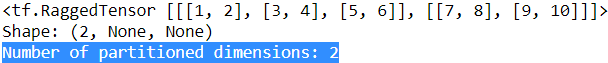
#y is 1x1, and the cell can broadcast according to # 2 x (r1) x 2 # and # x specifies that the number of partitions of the # values # tensor is ragged_rank=1
# x      (3d ragged):  2 x (r1) x 2
# y      (2d ragged):         1 x 1
# Result (3d ragged):  2 x (r1) x 2
x = tf.ragged.constant([ [[1, 2], [3, 4], [5, 6]],
                         [[7, 8]]
                       ],ragged_rank=1)
y = tf.constant([[10]])
print( (x+y).ragged_rank )# ==>1
print(x + y)
Why x can specify that the number of partitions of the underlying ^ values ^ tensor ((pylist is a ^ nested ^ list, tuple ^ or ^ np.ndarray)) is ragged_ rank=1? The nested element of since # x # values is a list with the same length = 2 (uniform inner dimension)
rt = tf.RaggedTensor.from_row_splits(
       #index=  0      1       2       3       4
    values=[ [1, 2], [3, 4], [5, 6], [7, 8] ],
    row_splits=[0, 3, 4]) # ==> [0,3), [3,4)
print(rt)
print("Shape: {}".format(rt.shape))
print("Number of partitioned dimensions: {}".format(rt.ragged_rank)) 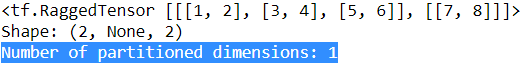
# x      (3d ragged):  2 x (r1) x (r2) x 1
# y      (1d tensor):                    3
# Result (3d ragged):  2 x (r1) x (r2) x 3
x = tf.ragged.constant([
                        [
                            [[1], [2]],
                            [],
                            [[3]],
                            [[4]],
                        ],
                        [
                            [[5], [6]],
                            [[7]]
                        ]
                       ],ragged_rank=2)
y = tf.constant([10, 20, 30])
# X broadcasting ==>2 x (r1) x (r2) x 3
# x = tf.ragged.constant([
#                         [
#                             [[1,1,1], [2,2,2]],
#                             [],
#                             [[3,3,3]],
#                             [[4,4,4]],
#                         ],
#                         [
#                             [[5,5,5], [6,6,6]],
#                             [[7,7,7]]
#                         ]
#                        ],ragged_rank=2)
print(x + y)
RaggedTensor coding
Irregular tensors are encoded using the # RaggedTensor # class. Internally, each raggedtenser contains:
- A , values , tensor that connects variable length rows into a flat list# [3, 1, 4, 1, 5, 9, 2]
- A row_partition, which indicates how to divide these flat values into rows# [0, 4, 4, 6, 7]
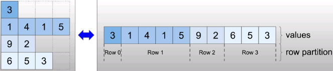 ==>
==>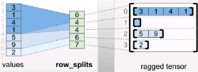
rt = tf.RaggedTensor.from_row_splits(
    values=[3, 1, 4, 1, 5, 9, 2],
    row_splits=[0, 4, 4, 6, 7])
print(rt)
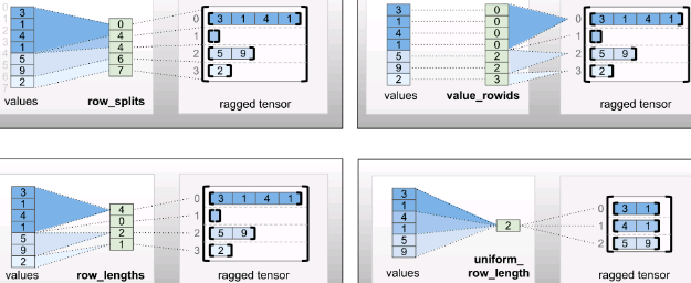
You can use four different encodings to store rows_ partition:
- row_splits is an integer vector used to specify the split point between rows: [start_index, end_index).
- value_rowids is an integer vector that specifies the row index for each value.
- row_lengths is an integer vector that specifies the length of each row.
- uniform_row_length is an integer scalar that specifies a single length for all rows.
 Integer scalar , nrows , can also be included in , row_partition , in the code to consider having , value_rowids' null trailing or has a uniform_ row_ Empty line of length.
Choosing which encoding to use for row partitioning is managed internally by irregular tensors to improve efficiency in some environments. In particular, some advantages and disadvantages of different row partition schemes are:
-
Efficient index: row_splits # coding can realize constant time indexing and slicing of irregular tensors.
-
Efficient connection: row_ Length encoding is more effective when connecting irregular tensors, because when two tensors are connected together, the line length does not change.
-
Smaller encoding size: value_rowids encoding is more effective when storing irregular tensors with a large number of empty rows, because the size of the tensor depends only on the total number of values. On the other hand, row_splits and rows_ Length encoding is more effective when storing irregular tensors with longer rows, because they require only one scalar value per row.
-
Compatibility: value_rowids scheme and TF segment_ Sum, etc subsection Format match. row_limits # scheme and tf.sequence_mask Match the format used by the operation.
-
Uniform dimension: as described below, uniform_row_length encoding is used to encode irregular tensors with uniform dimensions.
Multiple irregular dimensions
Irregular tensors with multiple irregular dimensions are encoded by using nested , RaggedTensor , for , values , tensors. Each nested , RaggedTensor , adds an irregular dimension.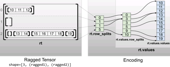
rt = tf.RaggedTensor.from_row_splits(
    values=tf.RaggedTensor.from_row_splits(
        #index:0  1   2   3   4   5   6   7   8   9   10
        values=[10, 11, 12, 13, 14, 15, 16, 17, 18, 19],#idx 0     1      2      3      4      5
        row_splits=[0, 3, 3, 5, 9, 10]),                 #==>[0,3), [3,3), [3,5), [5,9), [9,10)
    row_splits=[0, 1, 1, 5])                        #==>[0,1),[1,1),[1,                       5)
print(rt)
print("Shape: {}".format(rt.shape))
print("Number of partitioned dimensions: {}".format(rt.ragged_rank))
Factory function tf.RaggedTensor.from_nested_row_splits Can be used by providing a row_splits tensor list, directly construct raggedtenser with multiple irregular dimensions:
rt = tf.RaggedTensor.from_nested_row_splits(
    flat_values=[10, 11, 12, 13, 14, 15, 16, 17, 18, 19],
    nested_row_splits=([0, 1, 1, 5],       # second operation
                       [0, 3, 3, 5, 9, 10] # first operation
                      )
    )
print(rt)
print("Number of partitioned dimensions: {}".format(rt.ragged_rank))
Irregular rank sum flat value
The irregular rank of the irregular Tensor is the number of partitions of the underlying # values # Tensor (i.e. the nesting depth of the # RaggedTensor # object). The , values , Tensor of the innermost layer is called its , flat_values. In the following example, conversations {has ragged_ Its rank, flat = 3_ Values , is a one-dimensional , Tensor with 24 strings:
# shape = [batch, (paragraph), (sentence), (word)]
conversations = tf.ragged.constant(
     #b p s word_list
    [ [ [ ["I", "like", "ragged", "tensors."]
        ],
        [ ["Oh", "yeah?"],
          ["What", "can", "you", "use", "them", "for?"]
        ],
        [ ["Processing", "variable", "length", "data!"]
        ]
      ],
      [ [ ["I", "like", "cheese."],
          ["Do", "you?"]
        ],
        [ ["Yes."],
          ["I", "do."]
        ]
      ]
    ])

print( conversations.shape )
print("Number of partitioned dimensions: {}".format(conversations.ragged_rank) )
print("flat_values: ", conversations.flat_values)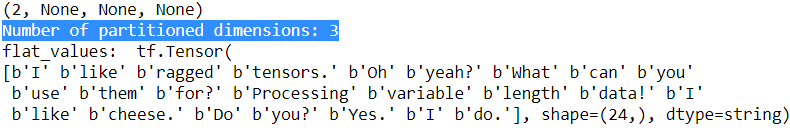
Uniform inner dimension
The irregular tensor with uniform inner dimension is flat_values (i.e. innermost} values) use multidimensional tf.Tensor Code.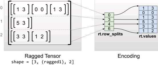
x is pylist: A nested list, tuple or NP ndarray. Bottom # values can be a # list, tuple # or # NP ndarray
rt = tf.RaggedTensor.from_row_splits(
    #index 0      1       2       3       4       5       6
    values=[[1, 3], [0, 0], [1, 3], [5, 3], [3, 3], [1, 2]],
    row_splits=[0, 3, 4, 6])
print(rt)
print("Shape: {}".format(rt.shape))
print("Number of partitioned dimensions: {}".format(rt.ragged_rank))
print("Flat values shape: {}".format(rt.flat_values.shape))
print("Flat values:\n{}".format(rt.flat_values)) 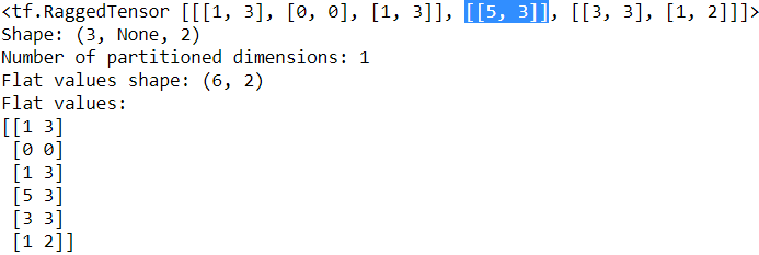
Uniform non inner dimension
Irregular tensors with uniform non inner dimensions are obtained by using {uniform_row_length encodes the row partition.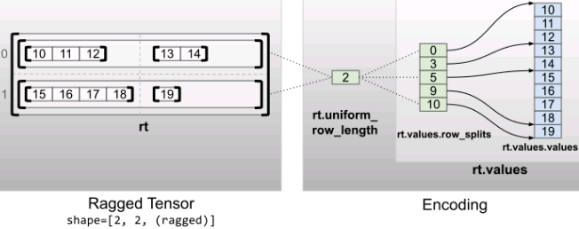
rt = tf.RaggedTensor.from_uniform_row_length(
    values=tf.RaggedTensor.from_row_splits(
        #index 0  1   2   3   4   5   6   7   8   9   10
        values=[10, 11, 12, 13, 14, 15, 16, 17, 18, 19],#idx 0           2             4
        row_splits=[0, 3, 5, 9, 10]),                   # ==>[0,3), [3,5), [5,9),[9,10)
    uniform_row_length=2)
print(rt)
print("Shape: {}".format(rt.shape))
print("Number of partitioned dimensions: {}".format(rt.ragged_rank))
inner_shape: a tuple of integers specifying the shape for individual inner values (the innermost values or bottom values tensor is called its flat_values) in the returned ragged tensor Defaults to () if ragged_rank is not specified. If ragged_rank is specified, then a default is chosen based on the contents of pylist
###########################https://www.tensorflow.org/guide/ragged_tensor?hl=zh-cn
We can now generate the dataset, with 50% good strings, and 50% bad strings:
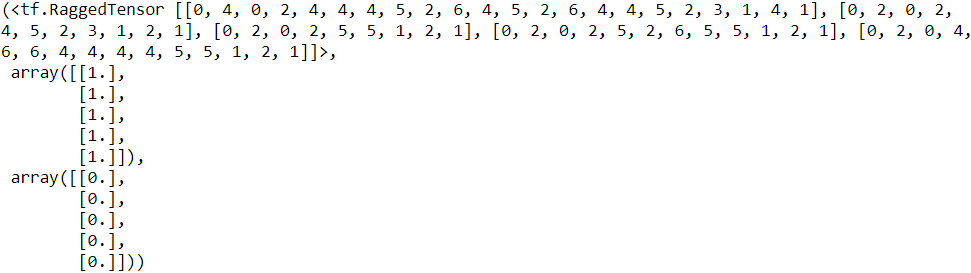
def generate_dataset(size):
    good_strings = [ string_to_ids(
                        generate_string(embedded_reber_grammar) #['string', 'string',...]
                     ) for _ in range(size//2) ] # [ [id,id,...], [id,,...], ... ]
    bad_strings = [ string_to_ids(
                        generate_corrupted_string(embedded_reber_grammar)
                    ) for _ in range(size-size//2) ]
    # all_strings is 2D
    all_strings = good_strings + bad_strings # '+': append operation
    # ragged_rank must be 1 since the innermost of all_strings is not uniform
    X = tf.ragged.constant( all_strings, ragged_rank=1 )
    y = np.array([ [1.] for _ in range( len(good_strings) )] +
                 [ [0.] for _ in range( len(bad_strings) ) ]
                )
    return X,y
np.random.seed(42)

X_train, y_train = generate_dataset( 10000 )
X_valid, y_valid = generate_dataset( 2000 )

X_train[:5], y_train[:5], y_train[-5:]
Let's take a look at the first training sequence:
X_train[0]

Perfect! We are ready to create the RNN to identify good strings. We build a simple sequence binary classifier:
####################################https://www.tensorflow.org/api_docs/python/tf/keras/layers/InputLayer
tf.keras.layers.InputLayer
ragged : Boolean, whether the placeholder created is meant to be ragged. In this case, values of 'None' in the 'shape' argument represent ragged dimensions. For more information about RaggedTensors, see this guide. Default to False.
####################################
from tensorflow import keras
# POSSIBLE_CHARS = "BEPSTVX"
np.random.seed(42)
tf.random.set_seed(42)
embedding_size = 5
# Ragged tensors can hold sequences of variable lengths
model = keras.models.Sequential([ # None: timesteps or input length
keras.layers.InputLayer( input_shape=[None], dtype=tf.int32, ragged=True ),
keras.layers.Embedding( input_dim=len(POSSIBLE_CHARS), # without oov
output_dim=embedding_size ),
keras.layers.GRU(30),
keras.layers.Dense(1, activation="sigmoid")
])
optimizer = keras.optimizers.SGD( lr=0.02, momentum=0.95, nesterov=True )
model.compile( loss="binary_crossentropy", optimizer=optimizer, metrics=["accuracy"] )
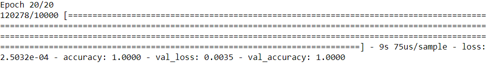
history = model.fit( X_train, y_train, epochs=20,
validation_data=(X_valid, y_valid) ) 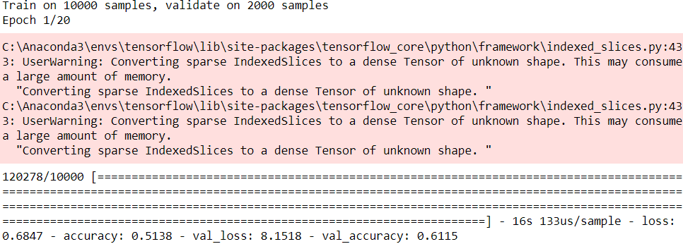
... ...
Now let's test our RNN on two tricky strings: the first one is bad while the second one is good. They only differ by the second to last character. If the RNN gets this right, it shows that it managed to notice the pattern that the second letter should always be equal to the second to last letter That requires a fairly long short-term memory (which is the reason why we used a GRU cell).
#
test_strings = ["BPBTSSSSSSSXXTTVPXVPXTTTTTVVETE",
"BPBTSSSSSSSXXTTVPXVPXTTTTTVVEPE"]
X_test = tf.ragged.constant([ string_to_ids(s) for s in test_strings ],
ragged_rank=1 )
y_proba = model.predict( X_test )
print()
print("Estimated probability that teste are Reber strings:")
for index, string in enumerate( test_strings ):
print( "{}: {:.2f}%".format(string, 100*y_proba[index][0]) ) 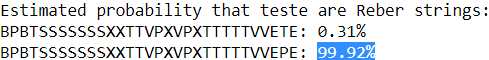 It worked fine. The RNN found the correct answers with very high confidence.
9. Train an Encoder–Decoder model that can convert a date string from one format to another (e.g., from "April 22, 2019" to "2019-04-22").
Let's start by creating the dataset. We will use random days between 1000-01-01 and 9999-12-31:
##########################
date.toordinal()
      Return the proleptic Gregorian ordinal of the date, where January 1 of year 1 has ordinal 1.
      For any date object d, date.fromordinal(d.toordinal()) == d.
from datetime import date dt=date.fromordinal( 1 ) print(dt) print( dt.strftime( "%d, %Y" ) ) print( dt.isoformat() )

##########################
from datetime import date

# cannot use strftime()'s %B format since it depends on the locale
MONTHS = ["January", "February", "March", "April", "May", "June",
          "July", "August", "September", "October", "November", "December"]
def random_dates( n_dates ):
    min_date = date(1000,1, 1).toordinal()
    max_date = date(9999, 12, 31).toordinal()

    ordinals = np.random.randint( max_date-min_date, size=n_dates ) + min_date
    dates = [ date.fromordinal( ordinal) for ordinal in ordinals ]
    x = [ MONTHS[dt.month-1] + " " + dt.strftime( "%d, %Y" ) for dt in dates ]
    y = [ dt.isoformat() for dt in dates ]
    return x, y
Here are a few random dates, displayed in both the input format and the target format:
np.random.seed(42)

n_dates = 3
x_example, y_example = random_dates( n_dates )
print( "{:25s}{:25s}".format("Input", "Target") )
print( "-"*50 )
for idx in range(n_dates):
print( "{:25s}{:25s}".format(x_example[idx], y_example[idx]) ) 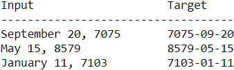
Let's get the list of all possible characters in the inputs:
INPUT_CHARS = "".join( sorted( set( "".join(MONTHS)
                                    + "0123456789, " )
                             ) )
INPUT_CHARS
And here's the list of possible characters in the outputs:
OUTPUT_CHARS = "0123456789-"
Let's write a function to convert a string to a list of character IDs, as we did in the previous exercise:
def date_str_to_ids( date_str, chars=INPUT_CHARS ):
    return [ chars.index(c) for c in date_str ]

date_str_to_ids(x_example[0], INPUT_CHARS)
date_str_to_ids( y_example[0], OUTPUT_CHARS )

def prepare_date_strs( date_strs, chars=INPUT_CHARS ):            #ragg #veriable length
    X_ids = [ date_str_to_ids(dt, chars) for dt in date_strs ]# [[nested_list],[nested_list]...]
    X = tf.ragged.constant( X_ids, ragged_rank=1 )
    return (X+1).to_tensor() # +1 for id start from 1

def create_dataset( n_dates ):
    x,y = random_dates(n_dates)
    return prepare_date_strs(x, INPUT_CHARS),\
           prepare_date_strs(y, OUTPUT_CHARS)
np.random.seed(42)

X_train, Y_train = create_dataset( 10000 )
X_valid, Y_valid = create_dataset( 2000 )
X_test, Y_test = create_dataset( 2000 )

Y_train[0]
 <=(X+1).to_tensor() # +1 for id start from 1<=
a very basic seq2seq model 1st version
Let's first try the simplest possible model: we feed in the input sequence, which first goes through the encoder (an embedding layer followed by a single LSTM layer), which outputs a vector, then it goes through a decoder (a single LSTM layer, followed by a dense output layer), which outputs a sequence of vectors, each representing the estimated probabilities for all possible output character.
Since the decoder expects a sequence as input, we repeat the vector (which is output by the decoder) as many times as the longest possible output sequence.
embedding_size = 32
max_output_length = Y_train.shape[1] # 10==len( "7075-09-20" )
np.random.seed(42)
tf.random.set_seed(42)
# INPUT_CHARS = ' ,0123456789ADFJMNOSabceghilmnoprstuvy'
encoder = keras.models.Sequential([
keras.layers.Embedding( input_dim=len(INPUT_CHARS)+1, #+1 since (X+1).to_tensor() # +1 for id start from 1
output_dim=embedding_size,
input_shape=[None] ),
keras.layers.LSTM(128) # return_sequences=False,
])# ==>(batch_size,128 ) just the last time step
# OUTPUT_CHARS = '0123456789-'
decoder = keras.models.Sequential([
keras.layers.LSTM( 128, return_sequences=True ),
keras.layers.Dense( len(OUTPUT_CHARS)+1, #+1 since (X+1).to_tensor() # +1 for id start from 1
activation="softmax" )
])
model = keras.models.Sequential([
encoder, #==>(batch_size,128 )
keras.layers.RepeatVector( max_output_length ),#==>(batch_size,max_output_length,128 )
decoder#==>(batch_size, max_output_length )
])
# https://blog.csdn.net/Linli522362242/article/details/113311720
# adam==>Nadam
optimizer = keras.optimizers.Nadam() # and the length of date string is veriable==>ragged tensor
model.compile( loss="sparse_categorical_crossentropy", # since OUTPUT_CHARS = "0123456789-"
optimizer=optimizer, metrics=["accuracy"] )
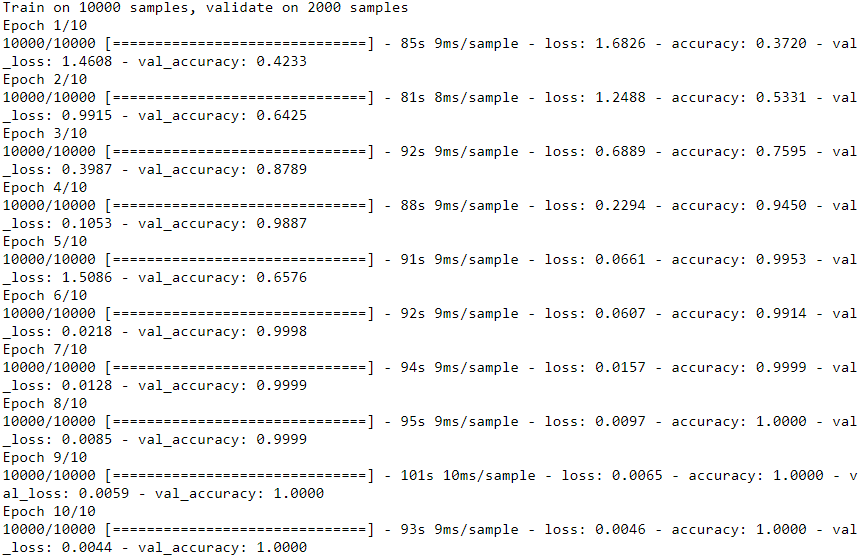
history = model.fit( X_train, Y_train, epochs=20,
validation_data=(X_valid, Y_valid) ) 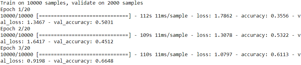
... ...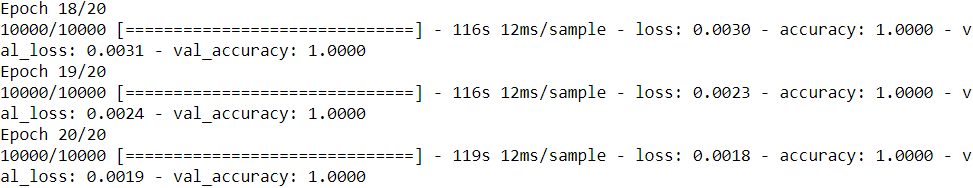 Looks great, we reach 100% validation accuracy!
model.summary()
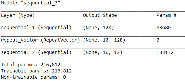
Let's use the model to make some predictions. We will need to be able to convert a sequence of character IDs to a readable string:
# def prepare_date_strs( date_strs, chars=INPUT_CHARS ):            #ragg #veriable length
#     X_ids = [ date_str_to_ids(dt, chars) for dt in date_strs ]# [[nested_list],[nested_list]...]
#     X = tf.ragged.constant( X_ids, ragged_rank=1 )
#     return (X+1).to_tensor() # +1 for id start from 1

# def create_dataset( n_dates ):
#     x,y = random_dates(n_dates)
#     return prepare_date_strs(x, INPUT_CHARS),\
#            prepare_date_strs(y, OUTPUT_CHARS)

#OUTPUT_CHARS = "0123456789-"
def ids_to_date_strs( ids, chars=OUTPUT_CHARS ):
                      # " " since (X+1).to_tensor() # +1 for id start from 1
    return [ "".join([ (" "+chars)[index] for index in sequence ])
             for sequence in ids ]
X_new = prepare_date_strs([ "September 17, 2009", "July 14, 1789" ])
# OR ids = model.predict_classes(X_new) 12<==since len("1789-07-14")
# model.predict(X_new).shape : (2, 10, 12) <==10<==since len("0123456789-")
ids = np.argmax( model.predict(X_new), axis=-1 )
for date_str in ids_to_date_strs(ids):
print(date_str) 
Perfect! :)
However, since the model was only trained on input strings of length 18 (which is the length of the longest date, e.g. len("September 17, 2009")==18), it does not perform well if we try to use it to make predictions on shorter sequences:
X_new = prepare_date_strs([ "May 02, 2020", "July 14, 1789" ])
#ids = model.predict_classes(X_new)
ids = np.argmax(model.predict(X_new), axis=-1)
for date_str in ids_to_date_strs(ids):
print(date_str)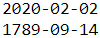 wrong! We need to ensure that we always pass sequences of the same length(same time steps) as during training, using padding if necessary. Let's write a little helper function for that:
X_train[19]

#####################################
tf.pad
https://www.tensorflow.org/api_docs/python/tf/pad
tf.pad(
    tensor, paddings, mode='CONSTANT', constant_values=0, name=None
)
"One" or "panic mode", fill
This operation pads a tensor according to the paddings you specify. paddings is an integer tensor with shape [n, 2], where n is the rank of tensor(Note: The rank of a tensor is not the same as the rank of a matrix. The rank of a tensor is the number of indices required to uniquely select each element of the tensor. Rank is also known as "order", "degree", or "ndims.").
# TF v2 style
def compute_z(a,b,c):
    r1 = tf.subtract(a,b)
    r2 = tf.multiply(2,r1)
    z = tf.add(r2,c)
    return z

tf.print('Scalar Inputs:', compute_z(1,2,3))
tf.print('Rank 1 Inputs:', compute_z([1], [2], [3]))
tf.print('Rank 2 Inputs:', compute_z([[1]], [[2]], [[3]]))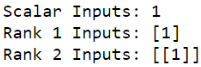
- For each dimension D of input, paddings[D, 0] indicates how many values to add before the contents of tensor in that dimension, and
- paddings[D, 1] indicates how many values to add after the contents of tensor in that dimension.
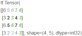
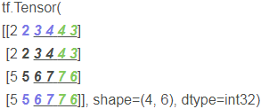
import tensorflow as tf

t=[[2,3,4],
   [5,6,7]
  ]

print(tf.pad(t,[[1,2], # [fill padding before d=0 OR axis=0 content, fill padding after d=0 OR axis=0 content]
                [3,4]  # [fill padding before d=1 OR axis=1 content, fill padding after d=1 OR axis=1 content]
               ],
              "CONSTANT")
)
tf.Tensor(
[[0 0 0 0 0 0 0 0 0 0]
[0 0 0 2 3 4 0 0 0 0]
[0 0 0 5 6 7 0 0 0 0]
[0 0 0 0 0 0 0 0 0 0]
[0 0 0 0 0 0 0 0 0]], shape = (5, 10), dtype = int32) # "CONSTANT"
Note: [1, 2] is the first one in pad, which represents the first dimension, that is, the row of matrix. 1 on the left represents 1 row 0 above and 2 on the right represents 2 rows 0 below
Similarly, the order of [3, 4] is the second, which represents column operation. 3 on the left represents putting 3 columns of 0 on the left, and 4 on the right represents putting 4 columns of 0 on the right
- If mode is "REFLECT" then both paddings[D, 0] and paddings[D, 1] must be no greater than tensor.dim_size(D) - 1.
import tensorflow as tf

t=[[2,3,4],
   [5,6,7]
  ]

print(tf.pad(t,[[1,2],
                [3,4]
               ],
              "REFLECT")
)
t.shape==2x2
Reason:
if D=0 ( OR axis=0 OR along to row), then both paddings[D, 0] and paddings[D, 1] must be no greater than tensor.dim_size(D)-1=2-1=1import tensorflow as tf t=[[2,3,4], [5,6,7] ] print(tf.pad(t,[[1,1], # d=0 OR axis=0, only 1 since t is 2x3, 2-1=1 [1,1] # d=1 OR axis=1,at most 2 since t is 2x3, 3-1=2 ], "REFLECT") )REFLECT
Turn up with 234 as the axis + turn down with 567 as the axis + turn left with vertical 5252 as the axis + turn right with vertical 7474 as the axis +
+ +
+ +
+
import tensorflow as tf

t=[[2,3,4],
   [5,6,7]
  ]

print(tf.pad(t,[[1,1],# d=0 OR axis=0
                [1,2] # d=1 OR axis=1, at most 2 since t is 2x3, 3-1=2
               ],
              "REFLECT")
)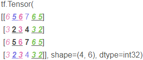
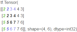
- If mode is "SYMMETRIC" then both paddings[D, 0] and paddings[D, 1] must be no greater than tensor.dim_size(D).
import tensorflow as tf

t=[[2,3,4],
   [5,6,7]
  ]

print(tf.pad(t,[[1,1],
                [1,2]
               ],
              "SYMMETRIC")
)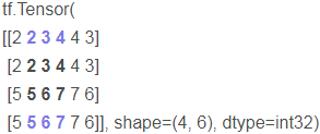
-
3D
import tensorflow as tf

t = tf.Variable(tf.ones([2, 3, 4]), name="tsr")
pad = np.array([[0, 0], # not fill padding on axis=0
                [1, 2], # fill padding on axis=1
                [3, 4]])# fill padding on axis=2

print(t)
print(tf.pad(t,pad,
              "CONSTANT")
)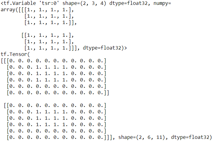
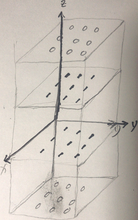
import tensorflow as tf t = tf.Variable(tf.ones([2, 3, 3]), name="tsr") pad = np.array([[1, 1], # fill padding on axis=0 [0, 0], # not fill padding on axis=1 [0, 0]])# not fill padding on axis=2 # print(t) print(tf.pad(t,pad, "CONSTANT") )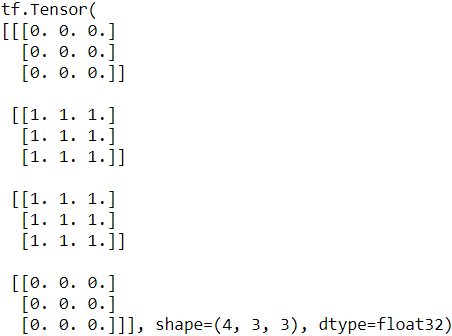 <==
<==
#####################################
X_train[19]

# since we use X = tf.ragged.constant( X_ids, ragged_rank=1 ) # Internal nonuniformity
max_input_length = X_train.shape[1] # 18


def prepare_date_strs_padded( date_strs ):
    X = prepare_date_strs( date_strs )
    if X.shape[1] <max_input_length:
        X = tf.pad(X, [ [ 0, 0 ],
                        [ 0, max_input_length-X.shape[1] ]
                      ])
    return X

def convert_date_strs( date_strs ):
    X = prepare_date_strs_padded( date_strs )
    # ids = model.predict_classes(X)
    ids = np.argmax( model.predict(X), axis=-1 ) # axis=-1(embedded dimension) for each character
    return ids_to_date_strs(ids)


convert_date_strs(["May 02, 2020",
"July 14, 1789"]) 
Cool! Granted, there are certainly much easier ways to write a date conversion tool (e.g., using regular expressions or even basic string manipulation), but you have to admit that using neural networks is way cooler. ;-)
However, real-life sequence-to-sequence problems will usually be harder, so for the sake of completeness, let's build a more powerful model.
feeding the shifted targets to the decoder (teacher forcing)-2nd version
Instead of feeding the decoder a simple repetition of the encoder's output vector, we can feed it the target sequence, shifted by one time step to the right. This way, at each time step the decoder will know what the previous target character was. This should help is tackle more complex sequence-to-sequence problems.
Since the first output character of each target sequence has no previous character, we will need a new token to represent the start-of-sequence (sos).
######################
sos_id = len(OUTPUT_CHARS) + 1
def shifted_output_sequences(Y):
sos_tokens = tf.fill( dims=(len(Y),1),
value=sos_id )
return tf.concat([ sos_tokens, Y[:,:-1] ],
axis=1 )
######################
During inference, we won't know the target, so what will we feed the decoder? We can just predict one character at a time, starting with an sos token, then feeding the decoder all the characters that were predicted so far.
#####################
since we use X = tf. ragged. Constant (x_ids, ragged_rank = 1) # internal non-uniform
max_input_length = X_train.shape[1] # 18
max_output_length = Y_train.shape[1]
def prepare_date_strs_padded( date_strs ):
X = prepare_date_strs( date_strs )
if X.shape[1] <max_input_length:
X = tf.pad(X, [ [ 0, 0 ],
[ 0, max_input_length-X.shape[1] ]
])
return X
sos_id = len(OUTPUT_CHARS)+1
def predict_date_strs( date_strs ):
X = prepare_date_strs_padded( date_strs )
Y_pred = tf.fill( dims=(len(X), 1), value=sos_id )
for index in range( max_output_length ):
pad_size = max_output_length - Y_pred.shape[1]
X_decoder = tf.pad(Y_pred, [[0,0], # not fill batch_size dimension
[0,pad_size] # fill sequence/timestep dimension for conver variable length sequence to fixed length(==max_output_length)
])
Y_probas_next = model.predict([X,X_decoder])[:, index:index+1]
Y_pred_next = tf.argmax( Y_probas_next, axis=-1, output_type=tf.int32 )
Y_pred = tf.concat([Y_pred, Y_pred_next], axis=1)
return ids_to_date_strs(Y_pred[:,1:])
#####################
But if the decoder's LSTM expects to get the previous target as input at each step, how shall we pass it it the vector output by the encoder? Well, one option is to ignore the output vector, and instead use the encoder's LSTM state as the initial state of the decoder's LSTM (which requires that encoder's LSTM must have the same number of units as the decoder's LSTM).
Now let's create the decoder's inputs (for training, validation and testing). The sos token will be represented using the last possible output character's ID + 1.
# def prepare_date_strs( date_strs, chars=INPUT_CHARS ): #ragg #veriable length
# X_ids = [ date_str_to_ids(dt, chars) for dt in date_strs ]# [[nested_list],[nested_list]...]
# X = tf.ragged.constant( X_ids, ragged_rank=1 )
# return (X+1).to_tensor() # +1 for id start from 1
# def create_dataset( n_dates ):
# x,y = random_dates(n_dates)
# return prepare_date_strs(x, INPUT_CHARS),\
# prepare_date_strs(y, OUTPUT_CHARS)
# np.random.seed(42)
# X_train, Y_train = create_dataset( 10000 )
# X_valid, Y_valid = create_dataset( 2000 )
# X_test, Y_test = create_dataset( 2000 )
sos_id = len(OUTPUT_CHARS) + 1
def shifted_output_sequences(Y):
sos_tokens = tf.fill( dims=(len(Y),1),
value=sos_id )
return tf.concat([ sos_tokens, Y[:,:-1] ],
axis=1 )
X_train_decoder = shifted_output_sequences(Y_train)
X_valid_decoder = shifted_output_sequences(Y_valid)
X_test_decoder = shifted_output_sequences(Y_test)
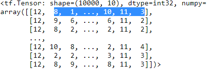
Y_train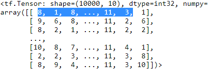 ==>shifted by one time step to the right
Let's take a look at the decoder's training inputs:
X_train_decoder
Now let's build the model. It's not a simple sequential model anymore, so let's use the functional API:
encoder_embedding_size = 32
decoder_embedding_size = 32
lstm_units = 128

np.random.seed(42)
tf.random.set_seed(42)
# INPUT_CHARS=' ,0123456789ADFJMNOSabceghilmnoprstuvy'
#     keras.layers.Embedding( input_dim=len(INPUT_CHARS)+1, #+1 since (X+1).to_tensor() # +1 for id start from 1
#                             output_dim=embedding_size,
#                             input_shape=[None] ),
encoder_input = keras.layers.Input( shape=[None], dtype=tf.int32 )
encoder_embedding = keras.layers.Embedding( input_dim=len(INPUT_CHARS)+1,#+1 since (X+1).to_tensor() # +1 for id start from 1
                                            output_dim=encoder_embedding_size
                                          )(encoder_input)
_, encoder_state_h, encoder_state_c = keras.layers.LSTM(
                                        lstm_units, return_state=True, # return_sequences=False,
                                      )(encoder_embedding)
encoder_state = [encoder_state_h, encoder_state_c]

# OUTPUT_CHARS = "0123456789-"
decoder_input = keras.layers.Input( shape=[None], dtype=tf.int32 )
decoder_embedding = keras.layers.Embedding( input_dim=len(OUTPUT_CHARS)+2,#+1 since +1 in (X+1).to_tensor() for id start from 1 and +1 again for sos
                                            output_dim=decoder_embedding_size
                                          )(decoder_input)
decoder_lstm_output = keras.layers.LSTM( lstm_units, return_sequences=True )(
                                         decoder_embedding, initial_state=encoder_state )
decoder_output = keras.layers.Dense( len(OUTPUT_CHARS)+1, #+1 since (X+1).to_tensor() # +1 for id start from 1 and we don't need to +1 again for predicting 'sos' with 0 probability
                                     activation="softmax" )(
                                     decoder_lstm_output )

model = keras.models.Model( inputs=[encoder_input, decoder_input],
                            outputs=[decoder_output] )
# https://blog.csdn.net/Linli522362242/article/details/113311720
# adam==>Nadam
optimizer = keras.optimizers.Nadam()# and the length of date string is veriable==>ragged tensor
model.compile( loss="sparse_categorical_crossentropy", # since OUTPUT_CHARS = "0123456789-"
               optimizer=optimizer,
               metrics=["accuracy"] )
history = model.fit( [X_train, X_train_decoder], Y_train,
                      epochs=10,
                      validation_data=([X_valid, X_valid_decoder], Y_valid)
                   )
This model also reaches 100% validation accuracy, but it does so even faster.
Let's once again use the model to make some predictions. This time we need to predict characters one by one.Figure 16-6. Neural machine translation using an Encoder–Decoder network with an attention model : https://blog.csdn.net/Linli522362242/article/details/115689038
# since we use X = tf.ragged.constant( X_ids, ragged_rank=1 ) # Internal nonuniformity
# max_input_length = X_train.shape[1] # 18
# max_output_length = Y_train.shape[1]

# def prepare_date_strs( date_strs, chars=INPUT_CHARS ):            #ragg #veriable length
#     X_ids = [ date_str_to_ids(dt, chars) for dt in date_strs ]# [[nested_list],[nested_list]...]
#     X = tf.ragged.constant( X_ids, ragged_rank=1 )
#     return (X+1).to_tensor() # +1 for id start from 1

# def prepare_date_strs_padded( date_strs ):
#     X = prepare_date_strs( date_strs )
#     if X.shape[1] <max_input_length:
#         X = tf.pad(X, [ [ 0, 0 ],
#                         [ 0, max_input_length-X.shape[1] ]
#                       ])
#     return X

sos_id = len(OUTPUT_CHARS)+1

def predict_date_strs( date_strs ):
    X = prepare_date_strs_padded( date_strs )
    Y_pred = tf.fill( dims=(len(X), 1), value=sos_id )
    for index in range( max_output_length ):
        pad_size = max_output_length - Y_pred.shape[1]
        X_decoder = tf.pad(Y_pred, [[0,0], # not fill batch_size dimension
                                    [0,pad_size] # fill sequence/timestep dimension
                                   ])

        Y_probas_next = model.predict([X,X_decoder])[:, index:index+1]
        Y_pred_next = tf.argmax( Y_probas_next, axis=-1, output_type=tf.int32 )
        Y_pred = tf.concat([Y_pred, Y_pred_next], axis=1)
    return ids_to_date_strs(Y_pred[:,1:])

predict_date_strs(["July 14, 1789", "May 01, 2020"])
Works fine!
using TF-Addons's seq2seq implementation(3rd version)
https://blog.csdn.net/Linli522362242/article/details/115518150
using TF-Addons's seq2seq implementation with a scheduled sampler(4th version)
https://blog.csdn.net/Linli522362242/article/details/115518150
using TFA seq2seq, the Keras subclassing API and attention mechanisms(5th version: )
The sequences in this problem are pretty short, but if we wanted to tackle longer sequences, we would probably have to use attention mechanisms. While it's possible to code our own implementation, it's simpler and more efficient to use TF-Addons's implementation instead. Let's do that now, this time using Keras' subclassing API.
Warning: due to a TensorFlow bug (see this issue https://github.com/tensorflow/addons/issues/1153 for details), the get_initial_state() method fails in eager mode, so for now we have to use the subclassing API, as Keras automatically calls tf.function() on the call() method (so it runs in graph mode).
In this implementation, we've reverted back to using the TrainingSampler, for simplicity (but you can easily tweak it to use a ScheduledEmbeddingTrainingSampler instead). We also use a GreedyEmbeddingSampler during inference, so this class is pretty easy to use:
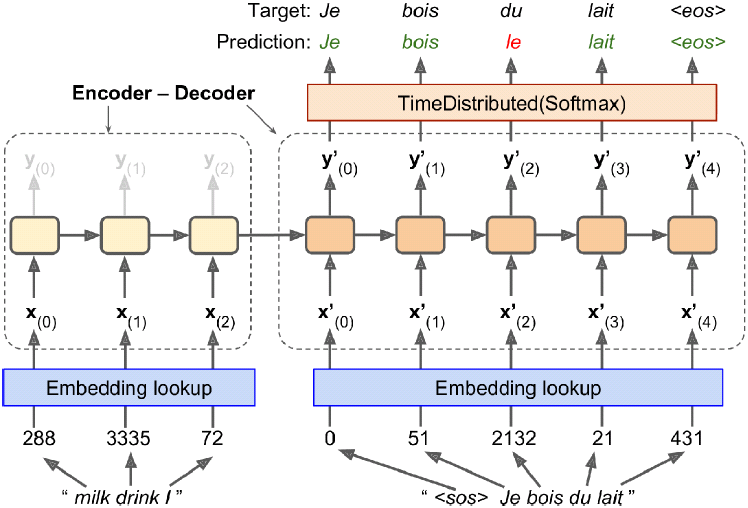 Figure 16-3. A simple machine translation model(just sending the encoder's final hidden state to the decoder)
Figure 16-6. Neural machine translation using an Encoder–Decoder network with an attention model
 is the alignment score vector. The decoder decides which part of the source sentence it needs to pay attention to, instead of having encoder encode all the information of the source sentence into a fixed-length vector.
 is the attention weight vector (=the number of time steps in encoder output) at the
  decoder time step. We apply a softmax activation function to the alignment scores to obtain the attention weights.
 is the attention Context Vector(=1x the number units in LSTMcell/GRUcell) at the the decoder time step.
The scaled dot-product attention of queries  , keys
 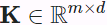 , and values
 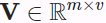 is
is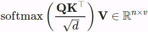
Note: Decoder receive (as input) : previous hidden state, all time steps of Encoder outputs, and previous time step Decoder output(inference time) OR previous time step target
Decoder LSTM/GRU
previous hidden state( OR encoder_final_state = [encoder_state_h, encoder_state_c] ), concatenation(+) between previous time step Decoder output(inference time) OR previous time step target(train time,after embedding lookup) + the scaled dot-product attention ( between previous hidden states and all time steps of Encoder outputs)
- cell_state : The state of the wrapped RNN cell at the previous time step t-1.
- attention(OR attention context) : the attention emitted at the previous time step t-1.
- Current time stored in time t
- alignments : A single or tuple of Tensor(s) containing the alignments emitted at the previous time step for each attention mechanism.
- alignment_history stores historical alignment information (if enabled) a single or multiple of tensorarray (s) containing alignment matrices from all time steps for each attention mechanism Call stack() on each to convert to a Tensor.
- attention_state : A single or tuple of nested objects containing attention mechanism state for each attention mechanism. The objects may contain Tensors or TensorArrays.
old version:
new version: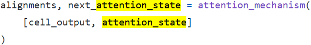 https://github.com/tensorflow/addons/blob/v0.12.0/tensorflow_addons/seq2seq/attention_wrapper.py#L1345-L1420
There is also a clone method in the AttentionWrapperState, which is also called in our model diagram: in fact, it is to initialize the AttentionWrapperState object to cell_ Replace the attribute value of state with the state output from the encoder (after average pooling). https://zhuanlan.zhihu.com/p/52608602
max_output_length = Y_train.shape[1]

class DateTranslation( keras.models.Model ):
  def __init__( self, units=128, encoder_embedding_size=32,
                decoder_embedding_size=32, **kwargs ):
    super().__init__(**kwargs)

    ################################# encoder
    self.encoder_embedding = keras.layers.Embedding(
        input_dim=len(INPUT_CHARS)+1, #+1 since (X+1).to_tensor() #+1 for id start from 1
        output_dim=encoder_embedding_size
    )
    self.encoder = keras.layers.LSTM( units,
                                      return_sequences=True,#will use an attention model(OR Alignment model)
                                      return_state=True # Whether to return the last state in addition to the output. Default: False
                                    )

    ################################# decoder
    self.decoder_embedding = keras.layers.Embedding(
        input_dim=len(OUTPUT_CHARS)+2,# +1 for id start from 1 and +1 again for 'SOS'
        output_dim=decoder_embedding_size
    )
    # https://blog.csdn.net/Linli522362242/article/details/115689038
    # https://github.com/tensorflow/addons/blob/v0.12.0/tensorflow_addons/seq2seq/attention_wrapper.py#L490-L609
    # def _calculate_attention(self, query, state):
    #     score = _luong_score(query, self.keys, self.scale_weight)
    #       # def _luong_score(query, keys, scale):
    #             # Reshape from [batch_size, depth] to [batch_size, 1, depth]
    #             # for matmul.
    #             query = tf.expand_dims(query, 1)
    #             score = tf.matmul(query, keys, transpose_b=True) # simply compute the dot product
    #             score = tf.squeeze(score, [1])#remove the dimension(=1) index at 1
    #             if scale is not None:
    #                 score = scale * score
    #     alignments = self.probability_fn(score, state)#probability_fn: str = "softmax",
    #     next_state = alignments
    #     return alignments, next_state
    # the attention mechanism is to measure the similarity between
    # one of the encoder's outputs and the decoder's previous hidden state
    # the encoder outputs (are both the keys and values)
    # the decoder hidden state at the decoder time step t-1 is the query
    # receive: the encoder outputs concatenated with the decoder's previous hidden state
    self.attention = tfa.seq2seq.LuongAttention(units) # (multiplicative)

    # why uses keras.layers.LSTMCell? During inference, we use one step output as next step input
    # keras.layers.LSTMCell processes one step within the whole time sequence input
    decoder_inner_cell = keras.layers.LSTMCell(units)# one time step or one word
    self.decoder_cell = tfa.seq2seq.AttentionWrapper(
                            cell=decoder_inner_cell,
                            attention_mechanism=self.attention
                          )# default output_attention: bool = True, the output at each time step is the attention value
    #+1 since (X+1).to_tensor() # +1 for id start from 1 and we don't need to +1 again for predicting 'sos' with 0 probability
    output_layer = keras.layers.Dense( len(OUTPUT_CHARS)+1)

    # https://www.tensorflow.org/addons/api_docs/python/tfa/seq2seq/TrainingSampler
    # A training sampler that simply reads its inputs.
    # its role is to tell the decoder at each step what it should pretend the
    # previous output was.
    # During inference, this should be the embedding of the token that was actually output
    # During training, it should be the embedding of the previous target token
    # time_major : Python bool. Whether the tensors in inputs are time major.
    #              If False (default), they are assumed to be batch major.
    # sampler = tfa.seq2seq.sampler.TrainingSampler()

    # In tfa.seq2seq.BasicDecoder
    # The tfa.seq2seq.Sampler instance passed as argument is responsible to
    # sample from the output distribution and
    # produce the input for the next decoding step.
    # https://www.tensorflow.org/addons/api_docs/python/tfa/seq2seq/BasicDecoder
    self.decoder = tfa.seq2seq.BasicDecoder(
        cell = self.decoder_cell, # contains LSTMCell and attention
        sampler = tfa.seq2seq.sampler.TrainingSampler(),
        output_layer = output_layer
    )

    # During inference, why GreedyEmbeddingSampler?
    # we've run the model(its input contains all previous outputs) once for each
    # new character if we use TrainingSampler
    # But,
    # at each time step, the GreedyEmbeddingSampler will compute the argmax of
    # the decoder's outputs, and run the resulting token IDs through the
    # decoder's embedding layer. Then it will feed the resulting embeddings to
    # the decoder's LSTM cell at the next time step. This way, we only need to
    # run the decoder once to get the full prediction.
    self.inference_decoder = tfa.seq2seq.BasicDecoder(
        cell = self.decoder_cell,# contains LSTMCell and attention
        sampler = tfa.seq2seq.sampler.GreedyEmbeddingSampler(
          embedding_fn = self.decoder_embedding
        ),
        output_layer = output_layer,
        maximum_iterations=max_output_length #prevent infinite loop
    )

  def call(self, inputs, training=None):         #None: num_time_steps
    # encoder_inputs = keras.layers.Input( shape=[None], dtype=np.int32 )
    # decoder_inputs = keras.layers.Input( shape=[None], dtype=np.int32 )
    encoder_input, decoder_input = inputs

    ################################# encoder
    encoder_embeddings = self.encoder_embedding(encoder_input)
    encoder_outputs, encoder_state_h, encoder_state_c = self.encoder(
                                                            encoder_embeddings,
                                                            training=training # **kwargs
                                                        )
    encoder_state = [encoder_state_h, encoder_state_c] # the last state
    # https://www.tensorflow.org/addons/api_docs/python/tfa/seq2seq/LuongAttention#setup_memory
    self.attention(encoder_outputs, # inputs shape: (None_batch_size, 18 time steps, 128 neurons
                   setup_memory=True)

    ################################# decoder
    decoder_embeddings = self.decoder_embedding( decoder_input )#shape: time steps x decoder_embedding_size
    # Luong attention(multiplicative) requires both vectors must have the same dimensionality
    # at each time step,
    # previous time step state(encoder_final_state) x target(OR time steps OR sequences)
    decoder_initial_state = self.decoder_cell.get_initial_state(
                                              decoder_embeddings # original state fields' shape
                            )# generate zero filled state for cell==> shape: decoder_embedding_size
    # https://www.tensorflow.org/addons/api_docs/python/tfa/seq2seq/AttentionWrapperState
    # clone
    # The new state fields' shape must match original state fields' shape.
    # This will be validated, and original fields' shape will be "propagated" to new fields.
    # print("decoder_initial_state",decoder_initial_state)            ###########
    decoder_initial_state = decoder_initial_state.clone(
                   # cell_state :
                   # The state of the wrapped RNN cell at the previous time step.
                                                  cell_state = encoder_state
                            )
    # print("decoder_initial_state after clone",decoder_initial_state) ###########
    if training:
        decoder_outputs, _, _ = self.decoder( decoder_embeddings,
                                              initial_state=decoder_initial_state,
                                              training=training )
    else:
        # sos_id = len(OUTPUT_CHARS) + 1 #==12
        start_tokens = tf.zeros_like( encoder_input[:, 0] )+sos_id
        # OR
        # batch_size = tf.shape(encoder_inputs)[:1]
        # start_tokens = tf.fill( dims=batch_size, value=sos_id )
        decoder_outputs, _, _ = self.inference_decoder(
            decoder_embeddings,
            initial_state=decoder_initial_state,
            start_tokens=start_tokens,
            end_token=0
        )
    # faster than keras.layers.Activation( "softmax" )( decoder_outputs.rnn_output )
    return tf.nn.softmax( decoder_outputs.rnn_output ) # Y_proba
decoder_initial_state AttentionWrapperState(cell_state=[<tf.Tensor 'date_translation_34/AttentionWrapperZeroState/checked_cell_state:0' shape=(None, 128) dtype=float32>,
<tf.Tensor 'date_translation_34/AttentionWrapperZeroState/checked_cell_state_1:0' shape=(None, 128) dtype=float32>
],
attention=<tf.Tensor 'date_translation_34/AttentionWrapperZeroState/zeros_3:0' shape=(None, 128) dtype=float32>,
alignments=<tf.Tensor 'date_translation_34/AttentionWrapperZeroState/zeros_2:0' shape=(None, 18) dtype=float32>, alignment_history=(),
attention_state=<tf.Tensor 'date_translation_34/AttentionWrapperZeroState/zeros_4:0' shape=(None, 18) dtype=float32>
)
decoder_initial_state after clone AttentionWrapperState(cell_state=[<tf.Tensor 'date_translation_34/Identity:0' shape=(None, 128) dtype=float32>,
<tf.Tensor 'date_translation_34/Identity_1:0' shape=(None, 128) dtype=float32>
],
attention=<tf.Tensor 'date_translation_34/Identity_2:0' shape=(None, 128) dtype=float32>,
alignments=<tf.Tensor 'date_translation_34/Identity_3:0' shape=(None, 18) dtype=float32>, alignment_history=(),
attention_state=<tf.Tensor 'date_translation_34/Identity_4:0' shape=(None, 18) dtype=float32>
)
np.random.seed(42)
tf.random.set_seed(42)

model = DateTranslation()
optimizer = keras.optimizers.Nadam()
model.compile( loss="sparse_categorical_crossentropy", optimizer=optimizer,
               metrics=["accuracy"] )
history = model.fit( [X_train, X_train_decoder], Y_train, epochs=25,
                     validation_data=([X_valid, X_valid_decoder], Y_valid)
                   )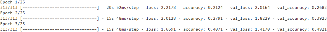
... ... Not quite 100% validation accuracy, but close. It took a bit longer to converge this time, but there were also more parameters and more computations per iteration. And we did not use a scheduled sampler.
To use the model, we can write yet another little function:
def ids_to_date_strs( ids, chars=OUTPUT_CHARS ):
                      # " " since we are using 0 as the padding token ID
    return [ "".join([ (" "+chars)[index] for index in sequence ])
             for sequence in ids ]

# since we use X = tf.ragged.constant( X_ids, ragged_rank=1 ) # Internal nonuniformity
max_input_length = X_train.shape[1] # 18

def prepare_date_strs_padded( date_strs ):
    X = prepare_date_strs( date_strs )
    if X.shape[1] <max_input_length:
        X = tf.pad(X, [ [ 0, 0 ],
                        [ 0, max_input_length-X.shape[1] ]
                      ])
    return X

def fast_predict_date_strs_v2( date_strs ):##############
  X = prepare_date_strs_padded( date_strs )
  # since the model require input([X_train, X_train_decoder])
  X_decoder = tf.zeros( shape=(len(X), max_output_length),
                        dtype=tf.int32 )
  Y_probas = model.predict( [X, X_decoder] )

  Y_pred = tf.argmax(Y_probas, axis=-1) # since tf.nn.softmax( decoder_outputs.rnn_output )
  return ids_to_date_strs(Y_pred)

fast_predict_date_strs_v2(["July 14, 1789", "May 01, 2020"])
There are still a few interesting features from TF-Addons that you may want to look at:
- Using a BeamSearchDecoder rather than a BasicDecoder for inference. Instead of outputing the character with the highest probability, this decoder keeps track of the several candidates, and keeps only the most likely sequences of candidates (see chapter 16 in the book for more details).
- Setting masks or specifying sequence_length if the input or target sequences may have very different lengths.
- Using a ScheduledOutputTrainingSampler, which gives you more flexibility than the ScheduledEmbeddingTrainingSampler to decide how to feed the output at time t to the cell at time t+1. By default it feeds the outputs directly to cell, without computing the argmax ID and passing it through an embedding layer. Alternatively, you specify a next_inputs_fn function that will be used to convert the cell outputs to inputs at the next step.
10. Go through TensorFlow's Neural Machine Translation with Attention tutorial.
Exercise: Go through TensorFlow's Neural Machine Translation with Attention tutorial : https://www.tensorflow.org/tutorials/text/nmt_with_attention.
Simply open the Colab and follow its instructions. Alternatively, if you want a simpler example of using TF-Addons's seq2seq implementation for Neural Machine Translation (NMT), look at the solution to the previous question. The last model implementation will give you a simpler example of using TF-Addons to build an NMT model using attention mechanisms.
This notebook trains a sequence to sequence (seq2seq) model for Spanish to English translation. This is an advanced example that assumes some knowledge of sequence to sequence models.
After training the model in this notebook, you will be able to input a Spanish sentence, such as "¿todavia estan en casa?", and return the English translation: "are you still at home?"
The translation quality is reasonable for a toy example, but the generated attention plot is perhaps more interesting. This shows which parts of the input sentence has the model's attention while translating: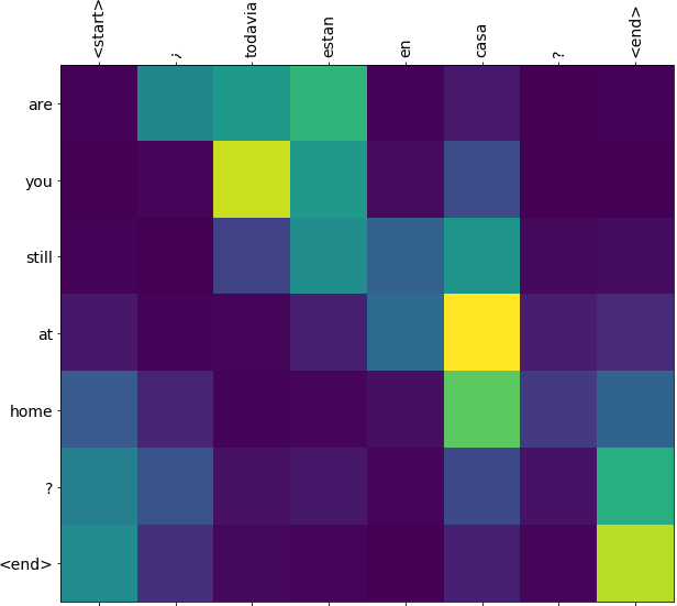
Download and prepare the dataset
We'll use a language dataset provided by http://www.manythings.org/anki/ This dataset contains language translation pairs in the format:
May I borrow this book? ¿Puedo tomar prestado este libro?
english sentence and spanish sentence is split with '\t'
There are a variety of languages available, but we'll use the English-Spanish dataset. For convenience, we've hosted a copy of this dataset on Google Cloud, but you can also download your own copy.
import os
import tensorflow as tf
# Download the file
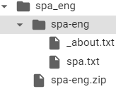
path_to_zip = tf.keras.utils.get_file(
fname='spa-eng.zip',
origin='http://storage.googleapis.com/download.tensorflow.org/data/spa-eng.zip',
cache_subdir="/content/drive/MyDrive/Colab Notebooks/data/spa_eng",
extract=True
)
path_to_file = os.path.dirname( path_to_zip ) + "/spa-eng/spa.txt"
https://docs.python.org/3/library/unicodedata.html
unicodedata.normalize(form, unistr)
Return the normal form form for the Unicode string unistr. Valid values for form are 'NFC', 'NFKC', 'NFD', and 'NFKD'.
The Unicode standard defines various normalization forms of a Unicode string, based on the definition of canonical [k əˈ n ɑ n ɪ kl] authoritative equivalence and compatibility equivalence In Unicode, several characters can be expressed in various way. For example, the character U+00C7 (LATIN CAPITAL LETTER C WITH CEDILLA) can also be expressed as the sequence U+0043 (LATIN CAPITAL LETTER C) U+0327 (COMBINING CEDILLA).
For each character, there are two Normal Forms: normal form C and normal form D.
- Normal form D (NFD) is also known as canonical decomposition, and translates each character into its decomposed form.
- Normal form C (NFC) first applies a canonical decomposition, then composes pre-combined characters again.
In addition to these two forms, there are two additional normal forms based on compatibility equivalence. In Unicode, certain characters are supported which normally would be unified with other characters. For example, U+2160 (ROMAN NUMERAL ONE) is really the same thing as U+0049 (LATIN CAPITAL LETTER I). However, it is supported in Unicode for compatibility with existing character sets (e.g. gb2312).
- The normal form KD (NFKD) will apply the compatibility decomposition, i.e. replace all compatibility characters with their equivalents.
- The normal form KC (NFKC) first applies the compatibility decomposition, followed by the canonical composition.
Even if two unicode strings are normalized and look the same to a human reader, if one has combining characters and the other doesn't, they may not compare equal.
unicodedata.category(chr)
Returns the general category assigned to the character chr as string.
After downloading the dataset, here are the steps we'll take to prepare the data:
- Add a start and end token to each sentence.
import unicodedata
import re

# Converts the unicode file to ascii
def unicode_to_ascii(s):
  # D (NFD) : translates each character into its decomposed form
  # "Mn" : Mark, Nonspacing https://blog.csdn.net/xc_zhou/article/details/82079753
  return ''.join( c for c in unicodedata.normalize('NFD', s)
                  if unicodedata.category(c) != "Mn"
                ) # for c in ... if ... then return c

def preprocess_sentence(w):
  # u"May I borrow this book?" ==> w.lower().strip() ==> "may i borrow this book?"
  # u"¿Puedo tomar prestado este libro?" ==> w.lower().strip() ==> "b'\xc2\xbfpuedo tomar prestado este libro?'"
  w = unicode_to_ascii( w.lower().strip() )

  # creating a space between a word and the punctuation following it
  # eg: "he is a boy." => "he is a boy ."
  # Reference:- https://stackoverflow.com/questions/3645931/python-padding-punctuation-with-white-spaces-keeping-punctuation
  # \1 : \one
  # "may i borrow this book?"  ==>
  # "may i borrow this book ? "
  # note: '\xc2\xbf' represents '¿'
  # "b'\xc2\xbfpuedo tomar prestado este libro?'"    ==>
  # "b' \xc2\xbf puedo tomar prestado este libro ? '"
  w = re.sub( r"([?.!,¿])", r" \1 ", w)

  # "may i borrow this book ? " ==>
  # "may i borrow this book ?"
  # "b' \xc2\xbf puedo tomar prestado este libro ? '" ==>
  # "b'\xc2\xbf puedo tomar prestado este libro ?'"
  w = w.strip()

  # adding a start and an end token to the sentence
  # so that the model know when to start and stop predicting.
  w = '<start> ' + w + ' <end>'
  return w
en_sentence = u"May I borrow this book?" sp_sentence = u"¿Puedo tomar prestado este libro?" print( preprocess_sentence(en_sentence) ) print( preprocess_sentence(sp_sentence).encode('utf-8') )
- Clean the sentences by removing special characters.
import io # 1. Remove the accents # 2. Clean the sentences # 3. Return word pairs in the format: [ENGLISH, SPANISH] def create_dataset( path, num_example ): lines = io.open( path, encoding='UTF-8' ).read().strip().split( '\n' ) word_pairs = [ [ preprocess_sentence(w) for w in line.split('\t') ] for line in lines[:num_example] ] return zip( *word_pairs ) en, sp = create_dataset( path_to_file, None ) print( en[0] ) print( sp[0] )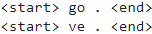 <==
<== 
- Create a word index and reverse word index (dictionaries mapping from word → id and id → word).
- Pad each sentence to a maximum length.
def tokenize( langSentence ):
  lang_tokenizer = tf.keras.preprocessing.text.Tokenizer( filters='',
                                                          char_level=False )
  lang_tokenizer.fit_on_texts( langSentence )

  tensor_seqs_indx=lang_tokenizer.texts_to_sequences( langSentence )
  # tf.keras.preprocessing.sequence.pad_sequences
  # maxlen
  #         Optional Int, maximum length of all sequences. If not provided,
  #         sequences will be padded to the length of the longest individual sequence.
  # padding
  #         String, 'pre' or 'post' (optional, defaults to 'pre'):
  #         pad either before or after each sequence.
  # value
  #         Float or String, padding value. (Optional, defaults to 0.)
  tensor_seqs_indx=tf.keras.preprocessing.sequence.pad_sequences( tensor_seqs_indx,
                                                                  padding='post'
                                                                )
  return tensor_seqs_indx, lang_tokenizer
Load dataset
def load_dataset( path, num_examples=None ):
  # creating cleaned input, output pairs
  # target: english; input: spanish
  targ_lang, inp_lang = create_dataset( path, num_examples )

  input_tensor, inp_lang_tokenizer = tokenize( inp_lang )
  target_tensor, targ_lang_tokenizer = tokenize( targ_lang )

  return input_tensor, target_tensor,\
         inp_lang_tokenizer, targ_lang_tokenizer
Limit the size of the dataset to experiment faster (optional)
Training on the complete dataset of >100,000 sentences will take a long time. To train faster, we can limit the size of the dataset to 30,000 sentences (of course, translation quality degrades with fewer data):
# Try experimenting with the size of that dataset
num_examples = 30000
# input: spanish; target: english
input_tensor, target_tensor,\
inp_lang_tokenizer, targ_lang_tokenizer = load_dataset( path_to_file,
                                                        num_examples )

# Calculate max_length of the target tensors
max_length_inp, max_length_targ = input_tensor.shape[1], target_tensor.shape[1]

max_length_inp, max_length_targ
from sklearn.model_selection import train_test_split

# Creating training and validation sets using an 80-20 split
input_train, input_val, target_train, target_val=train_test_split(input_tensor,
                                                                  target_tensor,
                                                                  test_size=0.2
                                                                 )
# Show length
print( len(input_train), len(target_train), len(input_val), len(target_val) )
def convert( lang_tokenizer, tensor ):
  for t in tensor:
    if t != 0: # since 0 : ' '
      print( f'{t} ----> {lang_tokenizer.index_word[t]}' )

print( "Input Language: index to word mapping" )
convert( inp_lang_tokenizer, input_train[0] )
print()
print( "Target Language: index to wrod mapping")
convert( targ_lang_tokenizer, target_train[0] )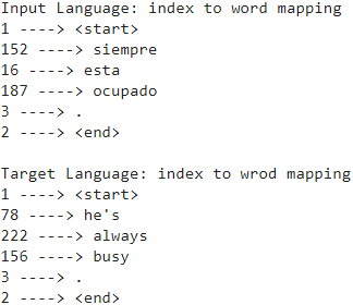
Create a tf.data dataset
BUFFER_SIZE = len( input_train )
BATCH_SIZE = 64
steps_per_epoch = len( input_train ) // BATCH_SIZE
embedding_dim = 256
units = 1024
vocab_inp_size = len( inp_lang_tokenizer.word_index )+1 # +1 for oov #9693
vocab_targ_size = len( targ_lang_tokenizer.word_index )+1            #5111

dataset = tf.data.Dataset.from_tensor_slices( (input_train, target_train)
                                            ).shuffle( BUFFER_SIZE )
dataset = dataset.batch( BATCH_SIZE, drop_remainder=True )

example_input_batch, example_target_batch = next( iter(dataset) )
example_input_batch.shape, example_target_batch.shape
Write the encoder and decoder model
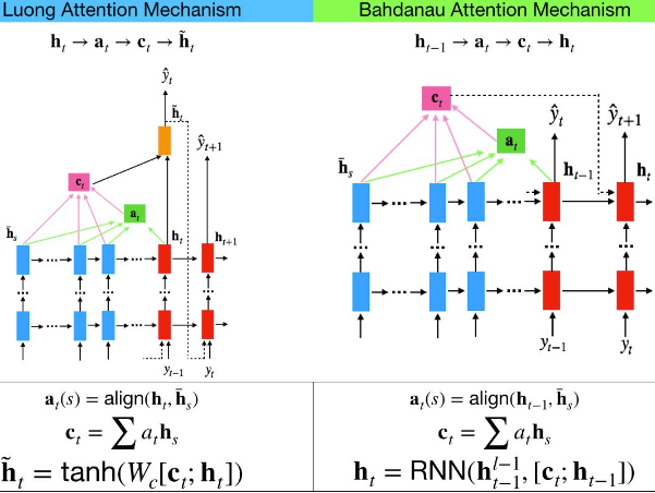
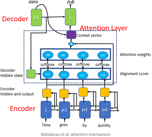
Implement an encoder-decoder model with attention which you can read about in the TensorFlow Neural Machine Translation (seq2seq) tutorial. This example uses a more recent set of APIs. This notebook implements the attention equations from the seq2seq tutorial. The following diagram shows that each input words is assigned a weight by the attention mechanism which is then used by the decoder to predict the next word in the sentence. The below picture and formulas are an example of attention mechanism from Luong's paper.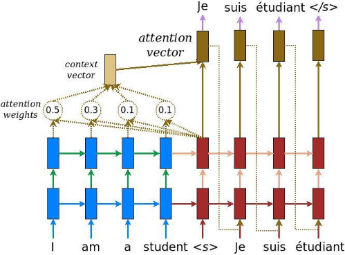
The input is put through an encoder model which gives us the encoder output of shape (batch_size, max_length of individual sequence, hidden_size=num_units) and the encoder hidden state of shape (batch_size, hidden_size==num_units).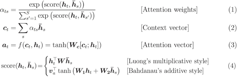
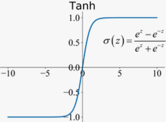
This tutorial uses Bahdanau attention for the encoder. Let's decide on notation before writing the simplified form:
- FC = Fully connected (dense) layer
- EO = Encoder output,
Encoder input : (batch_size, max_length of individual sequence)
==> embedding(vocab_size, embedding_dim) ==> (batch_size, max_length of individual sequence, embedding_dim)
==> (batch_size, max_length of individual sequence, embedding_dim) ==> GRU(units)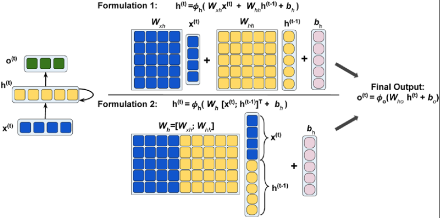 RNN
RNN
==> Encoder output : (batch_size, max_length of individual sequence, hidden_size=num_units) - H = hidden state
- X = input to the decoder
- Note: decoder_units==encoder_units since decoder GRUcell use encoder final hidden state (batch_size, self.enc_units) to initialize it in the beginning
and context_vector, attention_weights = self.attention( hidden_state, enc_output ), here hidden state is from previous time step (batch_size, self.dec_units)
And the pseudo-code:
- alignment score = FC( tanh( FC(EO) + FC(H) ) ) <==

- attention weights = softmax(score, axis = 1). Softmax by default is applied on the last axis but here we want to apply it on the 1st axis, since the shape of score is (batch_size, max_length of individual sequence, hidden_size==num_units). Max_length is the length of our input. Since we are trying to assign a weight to each input, softmax should be applied on that axis.
- context vector = sum(attention weights * EO, axis = 1). Same reason as above for choosing axis as 1.
shape : (batch_size, hidden_size==num_units==encoder RNN units == decoder RNN units) - embedding output = The input to the decoder X is passed through an embedding layer.
shape : X (batch_size, max_length of individual sequence) ==>one by one time step==> (batch_size, 1 time step)
==> embedding(vocab_size, embedding_dim)==> (batch_size, 1 time step, embedding_dim) - merged vector = concat(embedding output, context vector ==>expand_dims(context_vector, 1)
==>(batch_size, 1, hidden_size==num_units) )
==> concat ==> (batch_size, 1 , embedding_dim+ hidden_size==num_units) - This merged vector is then given to the GRU = 1 x GRUcell
(batch_size, 1, hidden_size=num_units) - ==> reshape ==> (batch_size, hidden_size=num_units) ==> fc=tf.keras.layers.Dense(vocab_size) ==> (batch_size, vocab_size)
The shapes of all the vectors at each step have been specified in the comments in the code: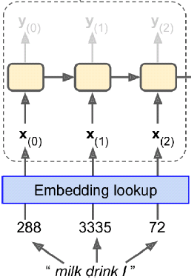
class Encoder(tf.keras.Model):
  def __init__(self, vocab_size, embedding_dim, enc_units, batch_sz):
    super(Encoder, self).__init__()
    self.batch_sz = batch_sz
    self.enc_units = enc_units

    self.embedding = tf.keras.layers.Embedding( input_dim=vocab_size,
                                                output_dim=embedding_dim
                                              )
    self.gru = tf.keras.layers.GRU( self.enc_units,
                                    return_sequences=True,
                                    return_state=True,
                                    recurrent_initializer='glorot_uniform'
                                  )

  def call(self, x, hidden):
    # x : (batch_size, max_length of individual sequence)
    x = self.embedding(x) # ==> (batch_size, max_length, embedding_dim)
    output, state = self.gru(x, initial_state=hidden)
    # output : (batch_size, max_length, self.enc_units)
    # final state : (batch_size, self.enc_units)
    return output, state

  def initialize_hidden_state(self):
    # encoder hidden state of shape : (batch_size, hidden_size==num_units)
    return tf.zeros( (self.batch_sz, self.enc_units) )
# vocab_inp_size = len( inp_lang_tokenizer.word_index )+1 # +1 for oov
# vocab_inp_size=9693, embedding_dim = 256, units = 1024, BATCH_SIZE = 64
encoder = Encoder(vocab_inp_size, embedding_dim, units, BATCH_SIZE)
# sample input
sample_hidden = encoder.initialize_hidden_state()
sample_output, sample_hidden_state = encoder(example_input_batch, sample_hidden)
print("Encoder output shape: (batch size, sequence length, units)", sample_output.shape)
print("Encoder Hidden state shape: (batch size, units)", sample_hidden.shape) 
class BahdanauAttention( tf.keras.layers.Layer ):
  def __init__(self, units):
    super(BahdanauAttention, self).__init__()
    self.W1 = tf.keras.layers.Dense(units)
    self.W2 = tf.keras.layers.Dense(units)
    self.V = tf.keras.layers.Dense(1)

  def call(self, query, values):
    # query(decoder previous hidden state) shape == (batch_size, hidden size)
    # we are doing this to broadcast addition along the time axis to calculate the score
    query_with_time_axis = tf.expand_dims( query, 1 )
    # query_with_time_axis shape == (batch_size, 1, hidden size)

    # values shape == (batch_size, max_len, hidden size==num_units) #from encoder output
    # we get 1 at the last axis because we are applying score to self.V
    #                         # + exists broadcasting
    score = self.V( tf.nn.tanh(self.W1(query_with_time_axis)+#==>(batch_size,1,units)
                               self.W2(values) #==>(batch_size,max_length,units)
                               )           # ==>(batch_size, max_length, units)
                  ) #==>alignment score shape : (batch_size, max_length, 1)
    # normalization
    attention_weights = tf.nn.softmax(score, axis=1)#==>(batch_size,max_length,1)

    # context_vector shape after sum == (batch_size, hidden_size)
    context_vector = attention_weights*values
    context_vector = tf.reduce_sum(context_vector, axis=1)#==>(batch_size, hidden_size==num_units)

    return context_vector, attention_weights
attention_layer = BahdanauAttention(10)
attention_result, attention_weights = attention_layer( sample_hidden,
sample_output )
print("Attention result shape: (batch size, units)", attention_result.shape )
print("Attention weights shape: (batch size, sequence_length, 1", attention_weights.shape )
class Decoder( tf.keras.Model ):
  def __init__( self, vocab_size, embedding_dim, dec_units, batch_sz ):
    super( Decoder, self ).__init__()
    self.batch_sz = batch_sz
    self.dec_units = dec_units
    self.embedding = tf.keras.layers.Embedding( vocab_size, embedding_dim )
    self.gru = tf.keras.layers.GRU( self.dec_units,
                                    return_sequences=True,
                                    return_state=True,
                                    recurrent_initializer='glorot_uniform' )
    self.fc = tf.keras.layers.Dense( vocab_size )

    # used for attention
    self.attention = BahdanauAttention( self.dec_units )
    # decoder_units==encoder_units since decoder GRUcell OR decoder's attention
    # use encoder final state in the begining

  def call( self, x, hidden, enc_output ):
    # x : target value(training time) OR decoder actual output(inference time)
    # enc_output shape == (batch_size, max_length, self.enc_units)
    # hidden : encoder final hidden state (batch_size, self.enc_units)
    # OR decoder previous time step hidden state (batch_size, self.dec_units)
    context_vector, attention_weights = self.attention( hidden, enc_output )
    #context_vector: (batch_size, hidden_size==num_units OR self.dec_units)

    # x shape (batch_size, 1 time step)
    x = self.embedding(x) # ==> (batch_size, 1, embedding_dim)

    x = tf.concat([ tf.expand_dims(context_vector,1), #==>(batch_size, 1, hidden_size==num_units)
                    x           # (batch_size, 1, embedding_dim)
                  ], axis=-1) #==>(batch_size, 1, embedding+hidden_size)
    # passing the concatenated vector to the GRU
    output, state = self.gru(x)
    # output : (batch_size, 1, hidden_size=self.dec_units)
    # current state : (batch_size, self.dec_units)

    # output shape == (batch_size * 1, hidden_size==self.dec_units)
    output = tf.reshape( output, (-1, output.shape[2]) )

    # output shape == (batch_size, target vocab size)
    x = self.fc(output)

    return x, state, attention_weights
decoder = Decoder( vocab_targ_size, embedding_dim, units, BATCH_SIZE )
# target value
sample_decoder_output, _, _ = decoder( tf.random.uniform( (BATCH_SIZE,1) ),
sample_hidden, # encoder final hidden state or decorder t-1 hidden state
sample_output )# encoder output sequences
print( "Decoder output shape: (batch_size, vocab size)", sample_decoder_output.shape ) 
Define the optimizer and the loss function
optimizer = tf.keras.optimizers.Adam()
# https://blog.csdn.net/Linli522362242/article/details/108414534
loss_object = tf.keras.losses.SparseCategoricalCrossentropy( from_logits=True,
                                                             reduction='none' )

def loss_function( real, pred ):
  # if real == 0 return True ==> logical_not ==> False ==> tf.cast ==>0.
  # if real == 1 return False ==> logical_not ==> True ==> tf.cast ==>1.
  mask = tf.math.logical_not( tf.math.equal(real,0) )
  loss_ = loss_object( real, pred )

  #https://blog.csdn.net/Linli522362242/article/details/115518150
  mask = tf.cast( mask, dtype=loss_.dtype )
  loss_ *= mask # to ignore the padding tokens(whose ID is 0) or
                # maskout time step whose value is padded with 0
                # so the masked time steps will not contribute to the loss (their loss will be 0)
  return tf.reduce_mean( loss_ )
Checkpoints (Object-based saving)
checkpoint_dir = '/content/drive/MyDrive/Colab Notebooks/checkpoints'
checkpoint_prefix = os.path.join( checkpoint_dir, "ckpt" )
checkpoint = tf.train.Checkpoint( optimizer=optimizer,
                                  encoder=encoder,
                                  decoder=decoder )
Training
- Pass the input through the encoder which return encoder output and the encoder hidden state.
- The encoder output, encoder hidden state(dec_hidden = enc_hidden) and the decoder input (which is the start token <start>) is passed to the decoder.
- The decoder returns the predictions and the decoder hidden state.
- The decoder hidden state is then passed back into the model and the predictions are used to calculate the loss.
- Use teacher forcing to decide the next input to the decoder.
- Teacher forcing is the technique where the target word is passed as the next input to the decoder.
- The final step is to calculate the gradients and apply it to the optimizer and backpropagate.
# tf.function
# https://blog.csdn.net/Linli522362242/article/details/107459161
@tf.function
def train_step(inp, targ, enc_hidden):
  loss = 0
  with tf.GradientTape() as tape:
    enc_output, enc_hidden = encoder(inp, enc_hidden)

    dec_hidden = enc_hidden
    # shift one step to right
    # OR dec_input = tf.expand_dims( targ[:,t], 1 ) # since first word is start token
    dec_input = tf.expand_dims( [targ_lang_tokenizer.word_index['<start>']
                                ]*BATCH_SIZE, 1)
    # Teacher forcing - feeding the target as the next input
    for t in range(1, targ.shape[1]):
      # passing enc_output to the decoder
      predictions, dec_hidden, _ = decoder(dec_input, dec_hidden, enc_output)

      loss += loss_function( targ[:, t], predictions )

      # using teacher forcing
      dec_input = tf.expand_dims( targ[:,t], 1 )

  batch_loss = ( loss/int(targ.shape[1]) )

  variables = encoder.trainable_variables + decoder.trainable_variables
  gradients = tape.gradient(loss, variables)

  optimizer.apply_gradients(zip(gradients, variables))

  return batch_loss
encoder.trainable_variables
# vocab_inp_size = len( inp_lang_tokenizer.word_index )+1 #==>9693=9692 words + 1 oov
# GRU( units =1024 )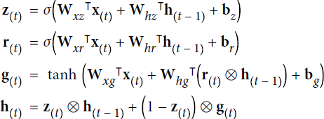 https://blog.csdn.net/Linli522362242/article/details/114941730
# tf.Variable encoder.trainable_variables:
- encoder/embedding/embeddings : shape=(input_dim=vocab_size==9693, # 9692 words + 1 oov
output_dim=embedding_dim==256) - encoder/gru/gru_cell/kernel for input : shape=(256=embedding_dim, 3072=W_x_reset(256, 1024 hidden units)+
W_x_update(256, 1024 hidden units)+
W_x_candidate(256, 1024 hidden units)) - for recurrent state
encoder/gru/gru_cell/recurrent_kernel : shape=(1024 hidden units, 3072=W_h_reset(1024 hidden units, 1024 hidden units)+
W_h_update(1024 hidden units, 1024 hidden units)+
W_h_candidate(1024 hidden units, 1024 hidden units)) - encoder/gru/gru_cell/bias : shape=(2 kernel, 3072=reset gate bias(1x1024 hidden units) +
update gate bias(1x1024 hidden units) +
candidate hidden state bias(1x1024 hidden units) )
decoder.trainable_variables
# vocab_targ_size = len( targ_lang_tokenizer.word_index )+1 #==>5111=5110 words + 1 oov
# GRU( units =1024 )
# Dense( vocab_size=5111 )
# tf.Variable decoder.trainable_variables:
- decoder/embedding_1/embeddings : shape=(input_dim=vocab_size==5111,
output_dim=embedding_dim==256) - decoder/gru_1/gru_cell_1/kernel : shape=(1280=embedding_dim+hidden_size=256+1024, 3072=1024*3)
- decoder/gru_1/gru_cell_1/recurrent_kernel : shape=(1024 units, 3072)
- decoder/gru_1/gru_cell_1/bias : shape=(2, 3072)
- #### output shape == (batch_size * 1, hidden_size==self.dec_units=1024 units)
decoder/dense_3/kernel : shape=(1024 units, 5111) - decoder/dense_3/bias : shape=(5111,)
###output shape == (batch_size, target vocab size= 5111)
decoder/bahdanau_attention_1/dense_4/kernel : shape=(1024, 1024)- decoder/bahdanau_attention_1/dense_4/bias : shape=(1024,)
- decoder/bahdanau_attention_1/dense_5/kernel : shape=(1024, 1024)
- decoder/bahdanau_attention_1/dense_5/bias : shape=(1024,)
- decoder/bahdanau_attention_1/dense_6/kernel : shape=(1024, 1)
- decoder/bahdanau_attention_1/dense_6/bias : shape=(1,)
import time

EPOCHS =10

for epoch in range(EPOCHS):
  start = time.time()

  enc_hidden = encoder.initialize_hidden_state() ###
  total_loss = 0
  # BUFFER_SIZE = len( input_train )
  # BATCH_SIZE = 64
  # steps_per_epoch = len( input_train ) // BATCH_SIZE =24000/64=375
  # dataset = tf.data.Dataset.from_tensor_slices( (input_train, target_train)
  #                                             ).shuffle( BUFFER_SIZE )
  # dataset = dataset.batch( BATCH_SIZE, drop_remainder=True )
  for (batch, (inp, targ)) in enumerate( dataset.take(steps_per_epoch) ):
    batch_loss = train_step( inp, targ, enc_hidden )
    total_loss += batch_loss

    if batch % 100 == 0:
      print( f'Epoch {epoch+1} Batch {batch} Loss {batch_loss.numpy():.4f}' )
  # saving (checkpoint) the model every 2 epochs
  if (epoch+1) % 2 ==0:
    checkpoint.save( file_prefix=checkpoint_prefix )

  print( f'Epoch {epoch+1} Loss {total_loss/steps_per_epoch:.4f}' )
print( f'Time taken for 1 epoch {time.time()-start:.2f} sec\n' ) 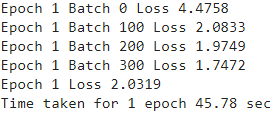
... ...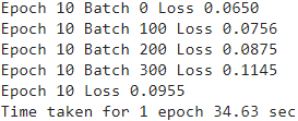
Translate
- The evaluate function is similar to the training loop, except we don't use teacher forcing here. The input to the decoder at each time step is its previous prediction(predicted_id = tf.argmax( predictions[0] ).numpy()) along with the hidden state and the encoder output.
- Stop predicting when the model predicts the end token.
- And store the attention weights for every time step.
import numpy as np

# units = 1024
def evaluate(sentence):
  # note: the batch_size should be 1 for only one sequence plotting
  attention_plot = np.zeros( (max_length_targ, max_length_inp) )
  sentence = preprocess_sentence(sentence)

  inputs = [ inp_lang_tokenizer.word_index[i] for i in sentence.split(' ') ]
  inputs = tf.keras.preprocessing.sequence.pad_sequences( [inputs], # extend dim to 2D (+batch_size dimension)
                                                          maxlen=max_length_inp,
                                                          padding='post'
                                                        )
  inputs = tf.convert_to_tensor( inputs )

  result = ''

  # initializes Decoder hidden state(gru cell including neuron units)
  hidden = [ tf.zeros( (1,units) ) ] #shape(1 time step, Encoder units==Decoder units)
  enc_out, enc_final_hidden = encoder( inputs, hidden )

  dec_hidden = enc_final_hidden
  dec_input = tf.expand_dims([ targ_lang_tokenizer.word_index['<start>']
                             ], 0) # 0 for appending a batch_size dimension
  for t in range( max_length_targ ):
    predictions, dec_hidden, attention_weights = decoder( dec_input,
                                                          dec_hidden,
                                                          enc_out )
    # storing the attention weights of decoder to plot later on
                      # (batch_size,max_length_inp,1) ==> (batch_size,max_length_inp*1)
    attention_weights = tf.reshape( attention_weights, (-1,) )
    attention_plot[t] = attention_weights.numpy() # batch_size must one

    # predictions shape(batch_size, vocab_targ_size) for current time step ############
    predicted_id = tf.argmax( predictions[0] ).numpy()

    result += targ_lang_tokenizer.index_word[predicted_id] + ' '

    if targ_lang_tokenizer.index_word[predicted_id] == '<end>':
      return result, sentence, attention_plot

    # the predicted ID is fed back into the model
    dec_input = tf.expand_dims([predicted_id],0) # 0 for appending a batch_size dimension

  return result, sentence, attention_plot
import matplotlib.pyplot as plt
import matplotlib.ticker as ticker
# function for plotting the attention weights
def plot_attention(attention, sentence, predicted_sentence):
fig = plt.figure( figsize=(10,10) )
ax = fig.add_subplot(1,1,1)
ms=ax.matshow( attention, cmap='viridis' )
fig.colorbar(ms)
fontdict = {'fontsize':14}
ax.set_xticklabels( ['']+sentence, fontdict=fontdict, rotation=90 )
ax.set_yticklabels( ['']+predicted_sentence, fontdict=fontdict )
ax.xaxis.set_major_locator( ticker.MultipleLocator(1) )
ax.yaxis.set_major_locator( ticker.MultipleLocator(1) )
plt.show()def translate( sentence ):
result, sentence, attention_plot = evaluate(sentence)
print('Input:', sentence)
print('Predicted translation:', result)
attention_plot = attention_plot[:len( result.split(' ') ),
:len( sentence.split(' ') )
]
plot_attention( attention_plot, sentence.split(' '), result.split(' ') )
# restoring the latest checkpoint in checkpoint_dir
checkpoint.restore( tf.train.latest_checkpoint( checkpoint_dir) )

translate(u'hace mucho frio aqui.')
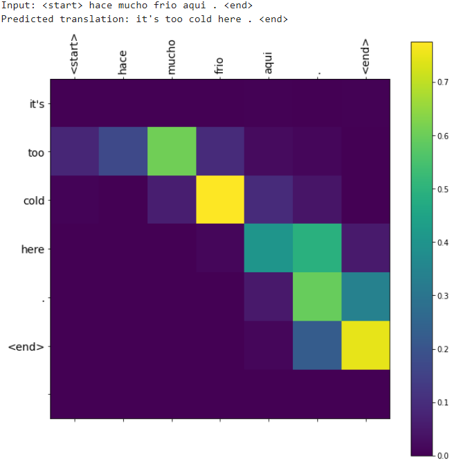
11. Use one of the recent language models (e.g., BERT) to generate more convincing Shakespearean text.
The simplest way to use recent language models is to use the excellent transformers library, open sourced by Hugging Face(https://huggingface.co/transformers/). It provides many modern neural net architectures (including BERT, GPT-2, RoBERTa, XLM, DistilBert, XLNet and more) for Natural Language Processing (NLP), including many pretrained models. It relies on either TensorFlow or PyTorch. Best of all: it's amazingly simple to use.
First, let's load a pretrained model. In this example, we will use OpenAI's GPT model https://huggingface.co/transformers/v2.0.0/pretrained_models.html, with an additional Language Model on top (just a linear layer with weights tied to the input embeddings). Let's import it and load the pretrained weights (this will download about 445MB of data to ~/.cache/torch/transformers):
!pip install transformers
from transformers import TFOpenAIGPTLMHeadModel

model = TFOpenAIGPTLMHeadModel.from_pretrained("openai-gpt")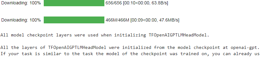
Next we will need a specialized tokenizer for this model. This one will try to use the spaCy and ftfy libraries if they are installed, or else it will fall back to BERT's BasicTokenizer followed by Byte-Pair Encoding (which should be fine for most use cases). https://huggingface.co/transformers/v2.0.0/model_doc/gpt.html
from transformers import OpenAIGPTTokenizer

tokenizer = OpenAIGPTTokenizer.from_pretrained("openai-gpt")
Now let's use the tokenizer to tokenize and encode the prompt text:
prompt_text = "This royal throne of kings, this sceptred isle"

encoded_prompt = tokenizer.encode( prompt_text, add_special_tokens=False,
                                   return_tensors="tf" )
encoded_prompt
tokenizer.convert_ids_to_tokens([ 616, 5751, 6404, 498, 9606, 240, 616, 26271, 7428, 16187])
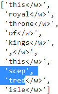
Easy! Next, let's use the model to generate text after the prompt. We will generate 5 different sentences, each starting with the prompt text, followed by 40 additional tokens. For an explanation of what all the hyperparameters do, make sure to check out this great blog post by Patrick von Platen (from Hugging Face https://huggingface.co/blog/how-to-generate). You can play around with the hyperparameters to try to obtain better results.
In transformers, we set do_sample=True and deactivate deactivate Top-K sampling (more on this later) via top_k=0. In the following, we will fix random_seed=0 for illustration purposes. Feel free to change the random_seed to play around with the model.
Fan et. al (2018) introduced a simple, but very powerful sampling scheme, called Top-K sampling. In Top-K sampling, the K most likely next words are filtered and the probability mass is redistributed among only those K next words. GPT2 adopted this sampling scheme, which was one of the reasons for its success in story generation.
After "The",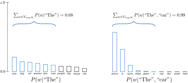 Having set K = 6, in both sampling steps we limit our sampling pool to 6 words. While the 6 most likely words, defined as
  encompass only ca. two-thirds of the whole probability mass in the first step, it includes almost all of the probability mass in the second step. Nevertheless, we see that it successfully eliminates the rather weird candidates
  in the second sampling step.
Top-p (nucleus) sampling
Instead of sampling only from the most likely K words, in Top-p sampling chooses from the smallest possible set of words whose cumulative probability exceeds the probability p. The probability mass is then redistributed among this set of words. This way, the size of the set of words (a.k.a the number of words in the set) can dynamically increase and decrease according to the next word's probability distribution. Ok, that was very wordy, let's visualize.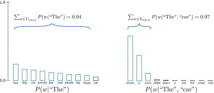 Having set p=0.92, Top-p sampling picks the minimum number of words to exceed together p=92% of the probability mass, defined as
  . In the first example, this included the 9 most likely words, whereas it only has to pick the top 3 words in the second example to exceed 92%. Quite simple actually! It can be seen that it keeps a wide range of words where the next word is arguably less predictable, e.g.
  , and only a few words when the next word seems more predictable, e.g.
  .
.
-
repetition_penalty can be used to penalize words that were already generated or belong to the context. It was first introduced by Kesker et al. (2019) and is also used in the training objective in Welleck et al. (2019). It can be quite effective at preventing repetitions, but seems to be very sensitive to different models and use cases, e.g. see this discussion on Github.
num_sequences = 5
length = 40
generated_sequences = model.generate(
    input_ids = encoded_prompt,
    do_sample=True,
    max_length = length + len(encoded_prompt[0]), #0 for sequence index in abatch
    temperature=1.0,
    top_k=0,
    top_p=0.9, # 0
    repetition_penalty=1.0,
    num_return_sequences=num_sequences,
)

generated_sequences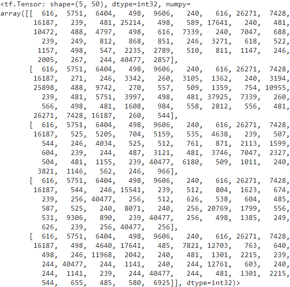
Now let's decode the generated sequences and print them:
for sequence in generated_sequences:
  text = tokenizer.decode( sequence, clean_up_tokenization_spaces=True )
  print(text)
  print('-'*80)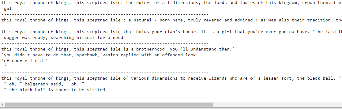
You can try more recent (and larger) models, such as GPT-2, CTRL, Transformer-XL or XLNet, which are all available as pretrained models in the transformers library, including variants with Language Models on top. The preprocessing steps vary slightly between models, so make sure to check out this generation example from the transformers documentation (this example uses PyTorch, but it will work with very little tweaks, such as adding TF at the beginning of the model class name, removing the .to() method calls, and using return_tensors="tf" instead of "pt".