Machine learning algorithms usually use cross validation techniques such as kFold to improve the accuracy of the model. In the process of cross validation, the prediction is carried out through the split test set that is not used for model training. These predictions are called out of fold predictions. External prediction plays an important role in machine learning and can improve the generalization performance of the model.
In this paper, we will introduce the discount prediction in machine learning, mainly including the following aspects:
- Out of sample prediction is a kind of out of sample prediction for data not used for training model.
- When predicting invisible data, discounted prediction is most commonly used to estimate the performance of the model.
- Discount prediction can be used to build integration model, which is called stack generalization or stack integration.
What is discount forecast?
Using resampling techniques such as k-fold to evaluate the performance of machine learning algorithms on data sets is a common method. The k-fold process includes dividing the training data set into k groups, and then using each of the K groups of samples as the test set, while the other samples are used as the training set.
This means that k different models were trained and evaluated. This process can be summarized as follows:
1. Randomly disrupt the data set.
2. Divide the dataset into k groups.
3. For each unique group: take this group as a reserved data for testing, take the remaining groups as the training data set, fit the model on the training set and evaluate it on the test set, repeat k times, so that each group of reserved data is tested.
4. Finally, the K models trained are used for integrated prediction.
Each data in the data sample is assigned to a separate group and remains in that group throughout the process. This means that each sample has the opportunity to be retained at least once as a test set and at most k-1 times as a training set. Discounted predictions are those made for each group of retained data (test set) during resampling. If performed correctly, each data in the training dataset will have a prediction.
The concept of discounted prediction is directly related to the concept of out of sample prediction, because the prediction in both cases is carried out on unused samples during model training, and the performance of the model in predicting new data can be estimated. Out of sample prediction is also an out of sample prediction, although it uses k-fold cross validation to evaluate the model.
Let's take a look at the two main functions of discount prediction
Evaluation of the model using discounted prediction
The most common use of discount prediction is to evaluate the performance of the model. Scoring indicators such as error or accuracy are used to predict and evaluate data not used for model training. It is equivalent to using new data (invisible data during training) for prediction and estimation of model performance. Using invisible data can evaluate the generalization performance of the model, that is, whether the model is over fitted.
Scoring the predictions made by the model during each training period and then calculating the average of these scores is the most commonly used model evaluation method. For example, if you have a classification model, you can calculate the classification accuracy on each group of predictions, and then estimate the performance as the average score of each group of discounted prediction estimates.
The following is a small example to show the model evaluation using discount prediction. First, use scikit learn's make_ The blobs () function creates a binary classification problem with 1000 samples, two classes, and 100 input features.
The following code prepares a data sample and prints the shapes of the input and output elements of the data set.
from sklearn.datasets import make_blobs
# create the inputs and outputs
X, y = make_blobs(n_samples=1000, centers=2, n_features=100, cluster_std=20)
# summarize the shape of the arrays
print(X.shape, y.shape)
Running this example will print the shape of the input data, display 1000 rows of data and 100 columns or input features and corresponding classification labels.
Next, KFold is used to group the data and train the kneigborsclassifier model.
We will use the parameter k=10 for KFold, which is a reasonable default value, fit a model on each group of data, and test and evaluate on the retained data of each group.
The scores are saved in the list of each model evaluation, and the average and standard deviation of these scores are printed.
# evaluate model by averaging performance across each fold
from numpy import mean
from numpy import std
from sklearn.datasets import make_blobs
from sklearn.model_selection import KFold
from sklearn.neighbors import KNeighborsClassifier
from sklearn.metrics import accuracy_score
# create the inputs and outputs
X, y = make_blobs(n_samples=1000, centers=2, n_features=100, cluster_std=20)
# k-fold cross validation
scores = list()
kfold = KFold(n_splits=10, shuffle=True)
# enumerate splits
for train_ix, test_ix in kfold.split(X):
# get data
train_X, test_X = X[train_ix], X[test_ix]
train_y, test_y = y[train_ix], y[test_ix]
# fit model
model = KNeighborsClassifier()
model.fit(train_X, train_y)
# evaluate model
yhat = model.predict(test_X)
acc = accuracy_score(test_y, yhat)
# store score
scores.append(acc)
print('> ', acc)
# summarize model performance
mean_s, std_s = mean(scores), std(scores)
print('Mean: %.3f, Standard Deviation: %.3f' % (mean_s, std_s))
Note: the results may vary due to the randomness of the algorithm or evaluation process or the difference of numerical accuracy. At the end of the run, the average and standard deviation of the printed scores are as follows:
>  0.95
>  0.92
>  0.95
>  0.95
>  0.91
>  0.97
>  0.96
>  0.96
>  0.98
>  0.91
Mean: 0.946, Standard Deviation: 0.023
In addition to averaging the prediction evaluation of each model, the prediction of each model can also be aggregated into a list, which contains the summary of the reserved data used as the test set during each group of training. After all model training, the list is taken as a whole to obtain a single accuracy score.
This method is used considering that each data appears only once in each test set. In other words, each sample in the training data set has a prediction in the cross validation process. So you can collect all the predictions and compare them with the target results, and calculate the score after the whole training. The advantage of this is that it can highlight the generalization performance of the model.
The complete code is as follows
# evaluate model by calculating the score across all predictions
from sklearn.datasets import make_blobs
from sklearn.model_selection import KFold
from sklearn.neighbors import KNeighborsClassifier
from sklearn.metrics import accuracy_score
# create the inputs and outputs
X, y = make_blobs(n_samples=1000, centers=2, n_features=100, cluster_std=20)
# k-fold cross validation
data_y, data_yhat = list(), list()
kfold = KFold(n_splits=10, shuffle=True)
# enumerate splits
for train_ix, test_ix in kfold.split(X):
# get data
train_X, test_X = X[train_ix], X[test_ix]
train_y, test_y = y[train_ix], y[test_ix]
# fit model
model = KNeighborsClassifier()
model.fit(train_X, train_y)
# make predictions
yhat = model.predict(test_X)
# store
data_y.extend(test_y)
data_yhat.extend(yhat)
# evaluate the model
acc = accuracy_score(data_y, data_yhat)
print('Accuracy: %.3f' % (acc))
All expected and predicted values of each retained dataset are printed with a single accuracy score at the end of the run.
Accuracy: 0.930
In addition to model evaluation, the biggest function of discount prediction is to integrate models and improve generalization ability.
Model integration with external forecast
Ensemble learning is a method of machine learning. It trains multiple models on the same training data, and integrates the predictions of multiple models to improve the overall performance. This is also the most common method in machine learning competitions.
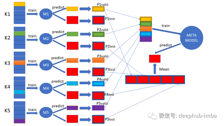
First, each model is cross validated and all discounted forecasts are collected. It should be noted that the data splitting performed by each model must be the same. In this way, we can get all the discount forecasts. In this way, the base model is obtained: the model evaluated by k-fold cross validation on the training data set, and all non folded predictions are retained.
Next, train a higher-order model (also known as meta model) according to the prediction of other models. The job of this model is to learn how to best combine and correct other models so that the discounted prediction of these (other) models can achieve better performance.
It sounds like a detour. Let's use a simple binary classification problem to explain. First, train a decision tree and a k-nearest neighbor model as the base model. Each base model predicts 0 or 1 for each sample in the training dataset through discounted prediction. These predictions are input into the meta model together with the input data.
- Meta model input: input characteristics of base model + prediction of base model.
- Meta model output: the target of the sample (the same as base models).
Why use discount prediction to train meta model?
Train the base model on the whole training data set, then predict each sample in the training data set, and use the prediction as the input of meta model. In this way, in fact, all samples are trained with meta model, and the prediction is certainly better than normal (it is very easy to produce over fitting), and meta model may not help to correct the base model prediction, It can even make the results worse.
However, meta model can be trained by using the discounted prediction of base model. Meta model can operate with the data invisible to base model, so as to obtain the deficiency of base model in predicting the behavior of new data, and correct the problem of base model through training. This is just like the case when integrated learning is used: all new data invisible during training are used.
Through cross validation, each base model is also trained on the whole data set, and these final base models and meta models can be used to predict new data. This process can be summarized as follows:
- For each base model, cross validation training is used and the discounted forecast is saved.
- Use the discount prediction in the base model to train the meta model.
This process is called stacked generalization, or stack for short. The linear weighted sum is usually used as the meta model, and this process is sometimes used ✌ It is called blending.
code implementation
This process can be described in detail here using the same data in the previous section. Firstly, the data is divided into training and verification data sets. The training data set will be used to fit the base model and meta model, and the validation data set will be used to evaluate the meta model and base model at the end of the training.
X, X_val, y, y_val = train_test_split(X, y, test_size=0.33)
The next step is to use cross validation to fit the DecisionTreeClassifier and kneigborsclassifier models of each discount and save the prediction outside the discount. These models will output probabilities rather than category labels because they need to provide more useful input features for meta models..
# collect out of sample predictions
data_x, data_y, knn_yhat, cart_yhat = list(), list(), list(), list()
kfold = KFold(n_splits=10, shuffle=True)
for train_ix, test_ix in kfold.split(X):
# get data
train_X, test_X = X[train_ix], X[test_ix]
train_y, test_y = y[train_ix], y[test_ix]
data_x.extend(test_X)
data_y.extend(test_y)
# fit and make predictions with cart
model1 = DecisionTreeClassifier()
model1.fit(train_X, train_y)
yhat1 = model1.predict_proba(test_X)[:, 0]
cart_yhat.extend(yhat1)
# fit and make predictions with cart
model2 = KNeighborsClassifier()
model2.fit(train_X, train_y)
yhat2 = model2.predict_proba(test_X)[:, 0]
knn_yhat.extend(yhat2)
The above code constructs a data set for meta model, which is composed of 100 input characteristics of input data and two prediction probabilities from kNN and decision tree model.
Create below_ meta_ The dataset () function takes the discounted data and forecast as the input, and constructs the input dataset for the meta model.
def create_meta_dataset(data_x, yhat1, yhat2):
# convert to columns
yhat1 = array(yhat1).reshape((len(yhat1), 1))
yhat2 = array(yhat2).reshape((len(yhat2), 1))
# stack as separate columns
meta_X = hstack((data_x, yhat1, yhat2))
return meta_X
This function is then called to prepare data for Meta-Model.
meta_X = create_meta_dataset(data_x, knn_yhat, cart_yhat)
Each base model is fitted to the whole training data set, and the validation set is used for prediction.
# fit final submodels
model1 = DecisionTreeClassifier()
model1.fit(X, y)
model2 = KNeighborsClassifier()
model2.fit(X, y)
Then meta model on the prepared data set, where we use logistic regression model.
# construct meta classifier
meta_model = LogisticRegression(solver='liblinear')
meta_model.fit(meta_X, data_y)
Finally, meta model is used to predict the retained data set. First, output the data set used to build the meta model through the base model, and then use the meta model for prediction. Encapsulate all these operations into a stack_ In the function of prediction().
# make predictions with stacked model
def stack_prediction(model1, model2, meta_model, X):
# make predictions
yhat1 = model1.predict_proba(X)[:, 0]
yhat2 = model2.predict_proba(X)[:, 0]
# create input dataset
meta_X = create_meta_dataset(X, yhat1, yhat2)
# predict
return meta_model.predict(meta_X)
Validation of the base model using the initially split retained dataset
# evaluate sub models on hold out dataset
acc1 = accuracy_score(y_val, model1.predict(X_val))
acc2 = accuracy_score(y_val, model2.predict(X_val))
print('Model1 Accuracy: %.3f, Model2 Accuracy: %.3f' % (acc1, acc2))
# evaluate meta model on hold out dataset
yhat = stack_prediction(model1, model2, meta_model, X_val)
acc = accuracy_score(y_val, yhat)
print('Meta Model Accuracy: %.3f' % (acc))
Merge all the above codes, and the complete code is as follows:
# example of a stacked model for binary classification
from numpy import hstack
from numpy import array
from sklearn.datasets import make_blobs
from sklearn.model_selection import KFold
from sklearn.model_selection import train_test_split
from sklearn.neighbors import KNeighborsClassifier
from sklearn.tree import DecisionTreeClassifier
from sklearn.linear_model import LogisticRegression
from sklearn.metrics import accuracy_score

# create a meta dataset
def create_meta_dataset(data_x, yhat1, yhat2):
# convert to columns
yhat1 = array(yhat1).reshape((len(yhat1), 1))
yhat2 = array(yhat2).reshape((len(yhat2), 1))
# stack as separate columns
meta_X = hstack((data_x, yhat1, yhat2))
return meta_X

# make predictions with stacked model
def stack_prediction(model1, model2, meta_model, X):
# make predictions
yhat1 = model1.predict_proba(X)[:, 0]
yhat2 = model2.predict_proba(X)[:, 0]
# create input dataset
meta_X = create_meta_dataset(X, yhat1, yhat2)
# predict
return meta_model.predict(meta_X)

# create the inputs and outputs
X, y = make_blobs(n_samples=1000, centers=2, n_features=100, cluster_std=20)
# split
X, X_val, y, y_val = train_test_split(X, y, test_size=0.33)
# collect out of sample predictions
data_x, data_y, knn_yhat, cart_yhat = list(), list(), list(), list()
kfold = KFold(n_splits=10, shuffle=True)
for train_ix, test_ix in kfold.split(X):
# get data
train_X, test_X = X[train_ix], X[test_ix]
train_y, test_y = y[train_ix], y[test_ix]
data_x.extend(test_X)
data_y.extend(test_y)
# fit and make predictions with cart
model1 = DecisionTreeClassifier()
model1.fit(train_X, train_y)
yhat1 = model1.predict_proba(test_X)[:, 0]
cart_yhat.extend(yhat1)
# fit and make predictions with cart
model2 = KNeighborsClassifier()
model2.fit(train_X, train_y)
yhat2 = model2.predict_proba(test_X)[:, 0]
knn_yhat.extend(yhat2)
# construct meta dataset
meta_X = create_meta_dataset(data_x, knn_yhat, cart_yhat)
# fit final submodels
model1 = DecisionTreeClassifier()
model1.fit(X, y)
model2 = KNeighborsClassifier()
model2.fit(X, y)
# construct meta classifier
meta_model = LogisticRegression(solver='liblinear')
meta_model.fit(meta_X, data_y)
# evaluate sub models on hold out dataset
acc1 = accuracy_score(y_val, model1.predict(X_val))
acc2 = accuracy_score(y_val, model2.predict(X_val))
print('Model1 Accuracy: %.3f, Model2 Accuracy: %.3f' % (acc1, acc2))
# evaluate meta model on hold out dataset
yhat = stack_prediction(model1, model2, meta_model, X_val)
acc = accuracy_score(y_val, yhat)
print('Meta Model Accuracy: %.3f' % (acc))
The complete code above first prints the accuracy of the decision tree and kNN model, and then prints the performance of the final meta model on the reserved dataset. It can be seen that the performance of the meta model is better than that of the two base models.
Model1 Accuracy: 0.670, Model2 Accuracy: 0.930
Meta-Model Accuracy: 0.955
It can be seen that although the accuracy of model 1 is only 67%, the integrated method of external prediction also has a good impact on the final result.
summary
- Out of sample prediction is a kind of out of sample prediction for data not used for training model.
- When predicting invisible data, discounted prediction is most commonly used to estimate the performance of the model.
- Discount prediction can also be used to build integration models, called stack generalization or stack integration.
https://www.overfit.cn/post/1ebf8320e9934d02ad74bafd198d67b5
By Jason Brownlee PhD